Overview
Abstract
The Circuit Solver was created to extract the lumped parameter physics calculations from within the individual systems and centralize the generic calculations. Closed loop circuits can be defined easily within the Common Data Model (CDM). They are fully dynamic, and can be manipulated and modified at each time step. The solver can be used to analyze electrical, fluid, and thermal circuits using native units. The solver outputs were validated using the outputs from an existing known third party circuit solver. All results matched the validation data, confirming this is a sound approach for the engine.
Introduction
Pulse systems use lumped parameter circuits to mimic the physiology of the human body. These circuits use fluid or thermal elements that are analogous to electrical circuit elements. The circuits have several types of feedback mechanisms that can be set and changed at every time step. Figure 1 presents a generic example of very low fidelity lumped parameter physiology circuits. Circuits can be thought of as pipe networks for fluid analysis.
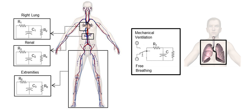 Figure 1 An example of physiology lumped parameter modeling. This example shows very low fidelity models of specific cardiovascular compartments (left), and a respiratory combined mechanical ventilation and free breathing model (right) [294].
Note: For simplicity, this document uses generic component/element terminology when discussing the solver functionality. See Table 1 for analogies and details about the mapping of electrical components.
The CDM includes many of the same generic definitions traditionally used to define and analyze circuits. Paths are ideal conductor branches that may contain elements (i.e., resistors, capacitors, inductors, diodes, etc.). Nodes are junctions at the intersection of paths. Figure 2 shows these base circuit element definitions. Paths are each assigned one source and one target node. We use the convention of positive current from source to target when performing calculations.
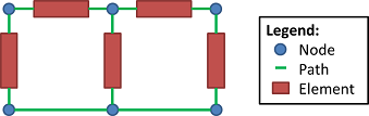 Figure 2 Nodes and paths are the lowest level elements used to define all circuits. Paths correspond to ideal conductors (i.e., wires). Nodes are placed at the intersections of paths. In fluid systems, paths can be thought of as frictionless pipes and nodes as pipe junctions.
System Design
Background and Scope
Requirements
In the Pulse engine, the major systems are modeled using circuit analogs with homeostatic feedback to mimic the physiology and pathophysiology of the human body. These circuits are made of fluid (liquid or gas) or thermal compartments modeled as electrical circuit components. In order to ease the implementation of individual system models and ensure adherence to sound physics principles, a generic circuit solver was created to centralize and solve the lumped-parameter circuit math. This generalized calculation ensures an accurate and consistent solution that can be reused for any models using circuit analogs. The circuit solver must provide modeling flexibility by allowing the addition, removal, and/or modification of circuit components each time-step during simulations. Therefore, DC transient analysis must be performed on nonlinear networks with the following high-level requirements:
- Generic - Leverageable by all physiological systems for rapid development and easy verification and validation (V&V)
- Multiphysics - Support simultaneous simulation of liquid, gas, and thermal circuits
- Comprehensive - Handle discrete passive components (i.e., wires, resistors, capacitors, inductors, switches, and diodes) and active components (i.e., voltage sources and current sources) with room for expansion
- Dynamic - Variable time-step and the ability to modify, add, or remove circuits, sub-circuits, components, and connections at run-time
- Modular - Support interdependent models for varying fidelity and complexity (e.g., multi-scale modeling) and aid in keeping systems decoupled
- Scalable - Able to efficiently solve any size network and connected networks
- Extensible - Reusable, repeatable, and interoperable implementation to allow for the addition of new capabilities and functionality
- Robust - Reliable computation of valid networks with extensive error handling
- Credible - Validated conservation of energy, mass, and momentum through a first principles implementation
- Efficient - Maintain full-body simulation faster than real-time with a shared dynamic time-step of 20 milliseconds
- Compatible - Reside within the C++ standardized data model (CDM) for ontologies and interfaces
- Comprehensible - Readable and understandable source code
- Open-Source - All software must adhere to Apache 2.0 license requirements
- Cross-Platform - Easy compilation and deployment for standard operating systems (Windows, Mac, Linux, and ARM)
Solutions Investigated
Early techniques for circuit simulation using computers were introduced in the 1950s, and several limited-scope simulators were developed [257]. The first general-purpose circuit simulator to experience widespread usage was SPICE (Simulation Program with Integrated Circuit Emphasis) coded in FORTRAN in the early 1970s. SPICE-based variations remain the most ubiquitous tools for circuit simulation software. There are several open-source successors, including XSPICE, CIDER, ngspice, and WRspice.
We considered several circuit solver options, including investigating existing software to determine if any would meet our needs. The best external code we found for integration into our C++ open source code was a variation on SPICE (Berkeley University’s Spice3f5), called Ngspice (http://ngspice.sourceforge.net/). Ngspice is an open source, general purpose circuit simulation program for nonlinear and linear analyses. It is developed with a C++ wrapper that maintains the original parametric netlist format (netlists can contain parameters and expressions) as inputs. During implementation, we found Ngspice to be a good fit for our needs to solve closed-loop circuits, yet several negatives forced us to deviate from that path. It was found to be very slow for our approach of solving a new (i.e., dynamic) circuit each time step. It was cumbersome to parse using the netlist input and output style. The most significant downside against implementing Ngspice into the engine was the unavoidable build-up of memory that caused our software to crash.
After evaluation, it was determined that none of the existing open-source simulators met all criteria required for a generic Pulse circuit solver. It would have taken significant effort to extract and modify the underlying code and overcome the limitations. Furthermore, many options examined have less permissive licensing requirements than Pulse. Therefore, we chose to create a tailored solution that is better suited to the specific needs of open-source physiology simulations.
Features and Capabilities
Approach and Extensibility
We created an analogical model that leverages the same standard network topology for all Pulse system types. Standardized circuits are defined in the CDM through paths connected by source and target nodes, similar to the netlists often used for electronic designs. Nodes hold information about the potential and quantity values and paths about the flux values. Paths can also include both passive and active components. Ideal resistances, capacitances, inductances, switches, diodes, potential sources, and flux sources are assignable to paths. There is no set number of paths assigned to each node, so the combinations of series and parallel components are limitless.
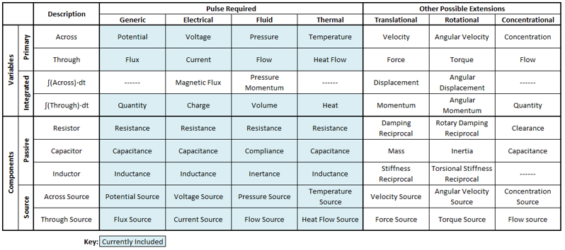
Table 1 shows the multiphysics mapping of circuit values across different domains. Mechanical (translational and rotational), fluid (liquid and gas), and thermal circuits are all defined. Our implementation uses the force-current and torque-current analogies. The resulting hydraulic equations that define fluid circuits approximately describe the relationship between a constant, laminar flow in a cylindrical pipe and the difference in pressure at each end. The reference/ground node is explicitly defined and the potential value can be set by the user for simulations that require ambient changes, like for the Pulse respiratory model that allows for altitude settings.
Table 1 The Pulse data model uses a templated approach to solve all circuit types with the same set of generic code. Highlighted cells were implemented as part of this work, while the other extensions can be easily added.
The circuit solver data model leverages C++ templates to allow operation with generic variables and component types using native electrical, fluid, and thermal units through the same logic. Conversions to and from base units are done in the background using the CDM unit conversion functionality. These base units are selected to prevent unnecessary conversion that would use critical computation resources, while still maintaining a direct mathematical relationship on both sides of the equation. The current and previous time-step values for all parameters are stored to allow transient analysis of time-dependent components (i.e., capacitances and inductances). Component values can be changed each time-step and can alternatively be added or removed at any time during the simulation. Nodes and paths can also be dynamically added or removed during simulation.
All three passive component types (resistors, capacitances, and inductances) have a polarized component modeling option for cases where reversed polarity is prohibited (e.g., elastic compartments that hold volume). When the target node potential becomes greater than that of the source node, polarized components act as a diode stopping all flux through the path. This allows the user to model electrolytic capacitors and further ensures fluid will not be added to hydraulic systems if compliances switch polarity.
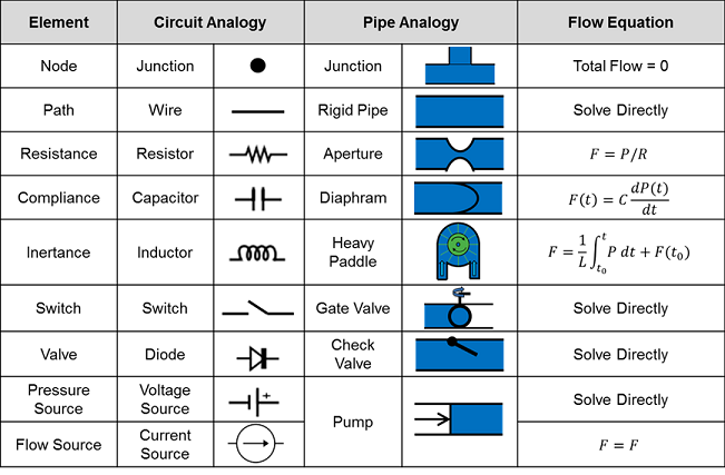
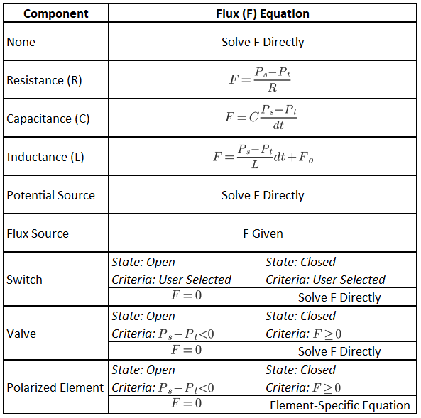
Further details specific to the implementation of our model with the hydraulic analogy are shown in Table 2. A more intuitive pipe analogy is described through images. The CDM defined fluid model elements are outlined in the first column. The flow equations are important for our analysis technique outlined earlier.
Table 2 In-depth description of the hydraulic analogy for electrical circuits that are used extensively inside the engine. The Elements are defined by the CDM and used by the solver. The Flow equations are important for solving for the unknown parameters. [401]
Black Box Implementation
Black box components have been designed in the circuit solver to allow for interfacing with external software or higher fidelity models. These 0-D black boxes have no knowledge of the internal workings of the component, but instead, act as a control volume with boundary conditions. The same source/target terminology is used as with all other circuit components, where the nodes act as the ports of the internal network. The two boundary potentials (source and target), two boundary fluxes (source and target), and one internal potential (middle) can be optionally imposed externally in any combination. All properties that are not imposed will be solved and set each time-step. Figure 3 shows the black box properties used by the solver.
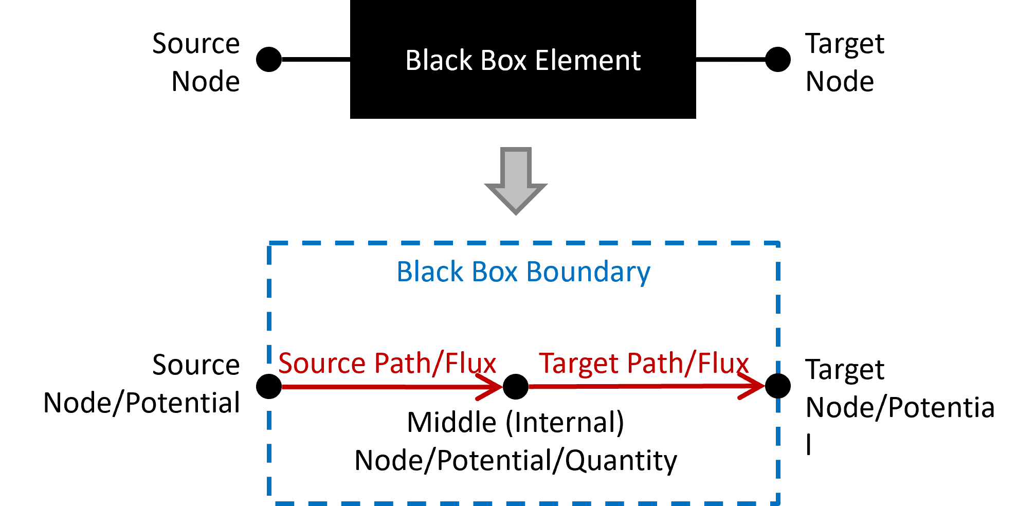
Internally, black box component imposed properties are applied in the circuit solver as potential or flux sources. A phantom path to ground is used for imposed potentials to determine the flow into/out of the black box. The internal/middle node is either explicitly set with an externally imposed potential value or calculated as the average of the source and target boundary potentials.
Black box compartments and links can be added to transport graphs for substance calculations the same as with any other circuit elements (see Substance Transport Methodology).
Data Model Implementation
Our CDM implementation and integration with physiological models is novel. We implemented the Circuit Solver to use generic terms that are not specific to any one model type (see Table 1). Conversions to base units for each model are done in the background using the CDM unit conversion functionality. These base units are selected to prevent unnecessary conversion that would use critical computation resources, while still maintaining a direct mathematical relationship on both sides of the equation when performing the calculations.
The CDM allows us to implement the circuit math in a completely modular fashion. Every system uses the same physics, with the same CDM-defined elements. The burden on system developers is merely in setting up and manipulating the circuit correctly. A benefit to using a CDM is a significantly reduced development time.
The only significant requirement for circuit design is that it must be closed-loop. Beyond that, the solver can handle any combination of valid nodes, paths, and elements. Only one (or zero) element is allowed on each path and the convention of positive current going from source node to target node is used.
This sound foundation for defining and calculating circuit parameters, allows the engine to transport substances in a similarly generic fashion (see Substance Transport Methodology).
Assumptions
Circuits
There are several assumptions made for the circuit math in general:
- All circuits must be closed-loop
- All elements are idealized
- All circuits must have a reference node defined with a known voltage - unlike other circuit solvers, it does not necessarily have to have a potential value of zero
- Nonlinear sources need initial values. Therefore, paths with capacitors that do not have an initial voltage on the source or target nodes will assign it the reference node voltage value, and paths with inductors that do not have an initial current will be assigned a value of zero.
Fluids
There are other assumptions specific to fluid systems:
- Flows are incompressible
- Fluids are inviscid
Limitations
While it is not necessarily a limitation, users of the Circuit Solver must be careful to assign current and voltage source elements to set currents and voltages respectively. Attempting to directly set node voltages or path currents would result in an over-constrained solution. In these instances, the solver will overwrite those values.
Data Flow
Our generic Circuit Solver intentionally mirrors the same data flow found in each of the systems. Each time step consists of a Preprocess call to set up the circuits for analysis, a Process call to do the analysis, and a Post Process call to advance the time in preparation for the next time step.
Preprocess
There is no literal Preprocess call within the circuit solver class (i.e., code). Each system individually and directly modifies its circuit(s). This allows our functionality to be entirely dynamic by performing a separate calculation every time step. See the Data Model Implementation Appendix below for details about CDM circuit elements and the data they contain.
Process
Network Analysis
Several mathematical methods for solving the state of the closed-loop circuit network were considered, including Sparse Tableau Analysis and nodal analysis. Ultimately, modified nodal analysis (MNA) was selected as the most advantageous approach. This technique leverages branch constitutive equations (i.e., potential-flux characteristics) and Kirkoff’s Laws to assemble the system and build the required network matrices. The key feature of MNA is assuming the sum of all path fluxes connected to each node is zero - inflows equal outflows. To achieve this balance, the solver iterates over all nodes contained in the circuit to generate a set of linear equations in the matrix form Ax=b. The matrix form of the solution is further defined by Equation 1, where G is the interconnections between passive components, B and C are the connections between potential sources, D is zero because only independent sources are considered, v and j are the potentials and fluxes, respectively, i is the sum of fluxes through passive components, and e is the independent potential sources [257].
![\[\left[ {\begin{array}{*{20}{c}} G&B\\ C&D \end{array}} \right]\left[ {\begin{array}{*{20}{c}} v\\ j \end{array}} \right] = \left[ {\begin{array}{*{20}{c}} i\\ e \end{array}} \right]\]](form_15.png)
After the MNA linear equations are solved, all node potentials and fluxes for paths with no components or source components are parsed out of the x vector. Path fluxes that are not directly determined at this stage are then calculated using the equations shown in Table 3.
Table 3 The flux equation on each path is dependent on what component is present. Some component types have their flux solved as direct variables using linear algebra. Some components are calculated differently depending on their state at that time. Ps and Pt are the source and target potentials respectively, dt is the time-step, and F0 is the previous time-step flux. Flux into a node is defined as positive and out is negative.
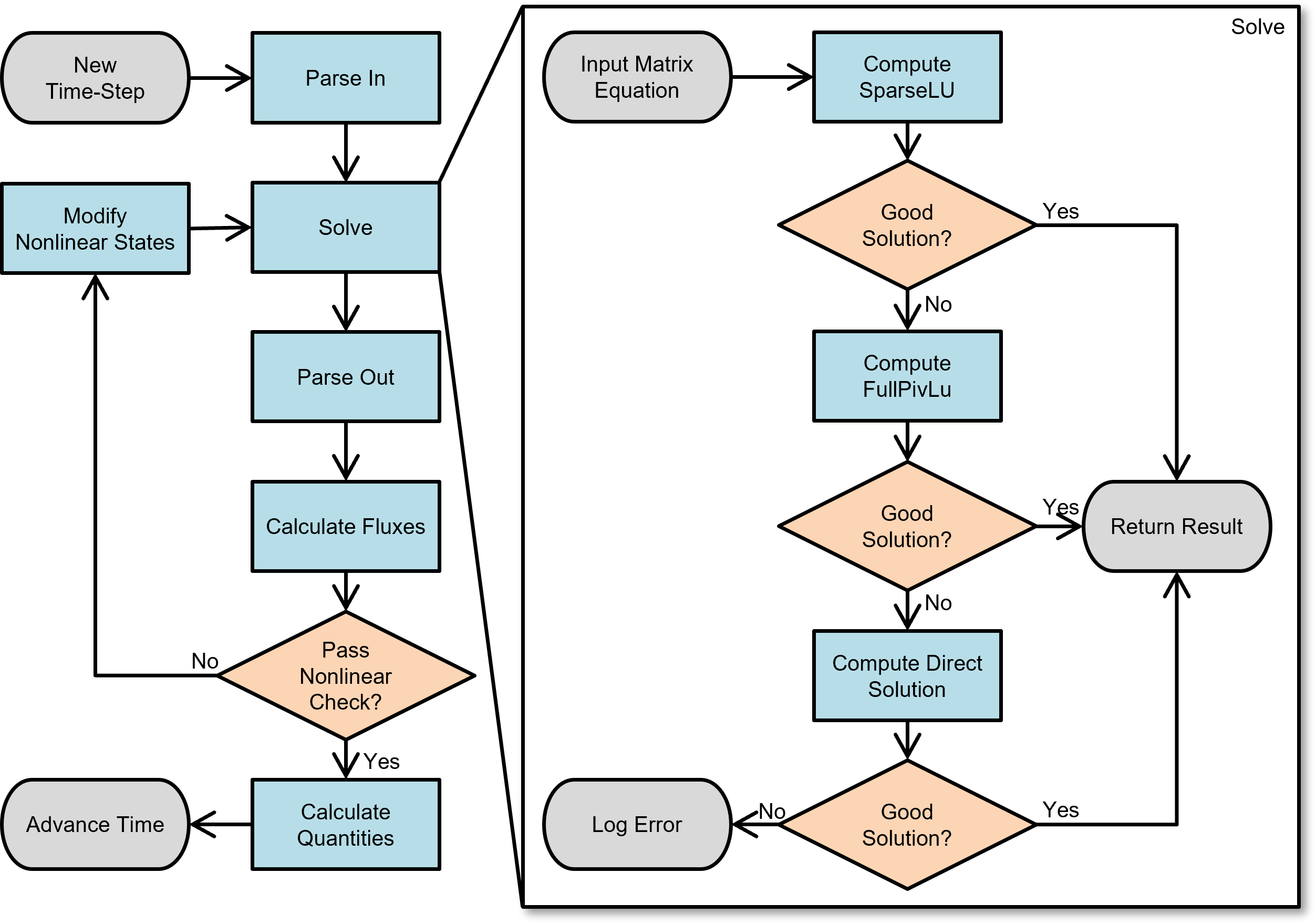
Quantity values (Q) on nodes that are connected to paths with capacitances are incremented by Equation 2, where Q0 is the previous quantity value. Figure 4 further illustrates this general circuit solver logic. The MNA matrices are rebuilt each time-step by parsing each node and iteratively populating the A matrix and x vector.
![\[Q = {Q_0} + F \cdot dt\]](form_16.png)
Linear Solver
The Pulse generic circuit solver leverages standard linear solver software. The b vector in Equation 1 is solved using methods provided by the Eigen open-source library for linear algebra. A number of algorithms within Eigen were tested for computationally efficient and accurate matrix solutions. The most efficient linear solver for most circumstances in Pulse was determined to be Sparse supernodal LU factorization (SparseLU). However, the circuit solver logic is designed to shift to the slower, but more robust LU decomposition with complete pivoting (FullPivLU) approach when SparseLU fails to provide accurate results. This logic is shown on the right side of Figure 4.
Nonlinear components (diodes and polarized components) have states with required behavior criteria, as shown in Table 3. These component states cannot be directly determined, but must be assumed and iteratively solved until a valid combination that meets all criteria is found. The conditional looping logic implemented in the circuit solver is shown on the left side of Figure 4.
There are several nuances for the handling of certain elements:
- Paths without elements are calculated as if they are zero voltage sources, which allows for direct solving for the current.
- Switches are modeled as elementless paths when closed and essentially infinite resistances (10100 ohms) when open.
- Valves (i.e., Diodes) are modeled as closed switches when the path source node voltage is higher than the target node (on) and as open switches when the voltage is greater on the target node (off).
- Polarized elements are modeled as an open switch when preventing polarity reversal
Post Process
Post Process effectively advances time by moving the “next” time step parameter values to the “current” time step parameter values (see System Methodology).
Results and Conclusions
Validation
Beyond several numerical (hand) calculations used during implementation, we performed validation on the generalized circuit math by duplicating circuits in LTspice (version 4.21s, created by Linear Technology, Milpitas, CA). LTspice is based on the well-documented and validated SPICE simulator. We created circuits using all elements individually and in combination. We used several different types of dynamically-changing drivers to ensure proper transient functionality. The resulting voltage and current values were interpolated and validated to match for all 114 circuits. Table 4 shows a summary of the validation circuits investigated.
Table 4 The list of circuits created in the engine and validated against LTspice. Every element is covered in combination with each other.
| Test Name | Purpose of test | Results Summary |
|---|---|---|
| BadDiodeDC | Intentionally failing to test Diode implementation | LTSpice: Will not run, Test: successfully fails - provides feedback on failure |
| BadDiodePULSE | Intentionally failing to test Diode implementation | LTSpice: Will not run, Test: successfully fails - provides feedback on failure |
| BadDiodeSIN | Intentionally failing to test Diode implementation | LTSpice: Will not run, Test: successfully fails - provides feedback on failure |
| BasicCircuit | Simple pressure source with resistances in series | Match |
| BasicDiodeDCCurrent | Diode behavior in response to a current source | Match |
| BasicDiodePULSECurrent | Diode behavior in response to a current source | Match |
| BasicDiodeSINCurrent | Diode behavior in response to a current source | Match |
| Comprehensive1DC | Combination of element types with a voltage source and a current source | Match |
| Comprehensive1PULSE | Combination of element types with a voltage source and a current source | Match |
| Comprehensive1SIN | Combination of element types with a voltage source and a current source | Match |
| CurrentCompDC | Combination of resistors and diode in response to a current source | Match |
| CurrentCompPulse | Combination of resistors and diode in response to a current source | Match |
| CurrentCompSIN | Combination of resistors and diode in response to a current source | Match |
| ParallelCapDC | Adding capacitors in parallel with a voltage source | Match |
| ParallelCapDCCurrent | Adding capacitors in parallel with a current source | Match |
| ParallelCapPulse | Adding capacitors in parallel with a voltage source | Match |
| ParallelCapPULSECurrent | Adding capacitors in parallel with a current source | Match |
| ParallelCapSIN | Adding capacitors in parallel with a voltage source | Match |
| ParallelCapSINCurrent | Adding capacitors in parallel with a current source | Match |
| ParallelCurrentSourceAdditionDC | Adding current sources in parallel | Match |
| ParallelCurrentSourceAdditionPULSE | Adding current sources in parallel | Match |
| ParallelCurrentSourceAdditionSIN | Adding current sources in parallel | Match |
| ParallelIndDC | Adding inductors in parallel with a voltage source | Match |
| ParallelIndDCCurrent | Adding inductors in parallel with a current source | Match |
| ParallelIndPULSE | Adding inductors in parallel with a voltage source | Match |
| ParallelIndPULSECurrent | Adding inductors in parallel with a current source | Match |
| ParallelIndSIN | Adding inductors in parallel with a voltage source | Match |
| ParallelIndSINCurrent | Adding inductors in parallel with a current source | Match |
| ParallelPressureSourceAdditionDC | Intentionally failing adding voltage sources in parallel | Test: successfully fails - provides feedback on failure |
| ParallelPressureSourceAdditionPULSE | Intentionally failing adding voltage sources in parallel | Test: successfully fails - provides feedback on failure |
| ParallelPressureSourceAdditionSIN | Intentionally failing adding voltage sources in parallel | Test: successfully fails - provides feedback on failure |
| ParallelRCDC | Parallel resistor and capacitor response to a voltage source | Match |
| ParallelRCPULSE | Parallel resistor and capacitor response to a voltage source | Match |
| ParallelRCSIN | Parallel resistor and capacitor response to a voltage source | Match |
| ParallelRDC | Parallel resistor response to a voltage source | Match |
| ParallelRDCCurrent | Parallel resistor response to a current source | Match |
| ParallelRLCDC | Parallel resistor, inductor, and capacitor response to a voltage source | Match |
| ParallelRLCDCCurrent | Parallel resistor, inductor and capacitor response to a current source | Match |
| ParallelRLCPULSE | Parallel resistor, inductor, and capacitor response to a voltage source | Match |
| ParallelRLCPULSECurrent | Parallel resistor, inductor and capacitor response to a current source | Match |
| ParallelRLCSIN | Parallel resistor, inductor, and capacitor response to a voltage source | Match |
| ParallelRLCSINCurrent | Parallel resistor, inductor and capacitor response to a current source | Match |
| ParallelRLDC | Parallel resistor and inductor response to a voltage source | Match |
| ParallelRLDCCurrent | Parallel resistor and inductor response to a current source | Match |
| ParallelRLPULSE | Parallel resistor and inductor response to a voltage source | Match |
| ParallelRLPULSECurrent | Parallel resistor and inductor response to a current source | Match |
| ParallelRLSIN | Parallel resistor and inductor response to a voltage source | Match |
| ParallelRLSINCentered | Parallel resistor and inductor response to a voltage source | Match |
| ParallelRLSINCurrent | Parallel resistor and inductor response to a current source | Match |
| ParallelRPULSE | Parallel resistor response to a voltage source | Match |
| ParallelRPulseCurrent | Parallel resistor response to a current source | Match |
| ParallelRSIN | Parallel resistor response to a voltage source | Match |
| ParallelRSINCurrent | Parallel resistor response to a current source | Match |
| SeriesCapDC | Adding capacitors in series with a voltage source | Match |
| SeriesCapDCCurrent | Adding capacitors in series with a current source | Match |
| SeriesCapPulse | Adding capacitors in series with a voltage source | Match |
| SeriesCapPULSECurrent | Adding capacitors in series with a current source | Match |
| SeriesCapSIN | Adding capacitors in series with a voltage source | Match |
| SeriesCapSINCurrent | Adding capacitors in series with a current source | Match |
| SeriesCurrentSourceAdditionDC | Intentionally failing adding current sources in series | Test: successfully fails - provides feedback on failure |
| SeriesCurrentSourceAdditionPULSE | Intentionally failing adding current sources in series | Test: successfully fails - provides feedback on failure |
| SeriesCurrentSourceAdditionSIN | Intentionally failing adding current sources in series | Test: successfully fails - provides feedback on failure |
| SeriesIndDC | Adding inductors in series with a voltage source | Match |
| SeriesIndDCCurrent | Adding inductors in series with a current source | Match |
| SeriesIndPULSE | Adding inductors in series with a voltage source | Match |
| SeriesIndPULSECurrent | Adding inductors in series with a current source | Match |
| SeriesIndSIN | Adding inductors in series with a voltage source | Match |
| SeriesIndSINCurrent | Adding inductors in series with a current source | Match |
| SeriesPressureSourceAdditionDC | Adding voltage sources in series | Match |
| SeriesPressureSourceAdditionPULSE | Adding voltage sources in series | Match |
| SeriesPressureSourceAdditionSIN | Adding voltage sources in series | Match |
| SeriesRCDC | Series resistor and capacitor response to a voltage source | Match |
| SeriesRCPULSE | Series resistor and capacitor response to a voltage source | Match |
| SeriesRCSIN | Series resistor and capacitor response to a voltage source | Match |
| SeriesRDC | Series resistors response to a voltage source | Match |
| SeriesRLCDC | Series resistor, inductor and capacitor response to a voltage source | Match |
| SeriesRLCDCCurrent | Series resistor, inductor and capacitor response to a current source | Match |
| SeriesRLCPULSE | Series resistor, inductor and capacitor response to a voltage source | Match |
| SeriesRLCPULSECurrent | Series resistor, inductor and capacitor response to a current source | Match |
| SeriesRLCSIN | Series resistor, inductor and capacitor response to a voltage source | Match |
| SeriesRLCSINCurrent | Series resistor, inductor and capacitor response to a current source | Match |
| SeriesRLDC | Series resistor and inductor response to a voltage source | Match |
| SeriesRLDCCurrent | Series resistor and inductor response to a current source | Match |
| SeriesRLPULSE | Series resistor and inductor response to a voltage source | Match |
| SeriesRLPULSECurrent | Series resistor and inductor response to a current source | Match |
| SeriesRLSIN | Series resistor and inductor response to a voltage source | Match |
| SeriesRLSINCurrent | Series resistor and inductor response to a current source | Match |
| SeriesRPULSE | Series resistors response to a voltage source | Match |
| SeriesRSIN | Series resistors response to a voltage source | Match |
| SimpleDiodeDC | Diode behavior in response to a voltage source | Match |
| SimpleDiodePULSE | Diode behavior in response to a voltage source | Match |
| SimpleDiodeSIN | Diode behavior in response to a voltage source | Match |
| SwitchRCDC | Circuit behavior when a switch is thrown with a voltage source | Match |
| SwitchRCDCCurrent | Circuit behavior when a switch is thrown with a current source | Match |
| SwitchRCPULSE | Circuit behavior when a switch is thrown with a voltage source | Match |
| SwitchRCPULSECurrent | Circuit behavior when a switch is thrown with a current source | Match |
| SwitchRCSIN | Circuit behavior when a switch is thrown with a voltage source | Match |
| SwitchRCSINCurrent | Circuit behavior when a switch is thrown with a current source | Match |
The most interesting and complex circuits use a combination of all elements. Two of these comprehensive circuits are shown below because of their complexity. The first uses sine wave sources and the second uses pulse sources. There is a strong correlation between the given LTspice outputs and the calculated outputs. Note that the sign convention of the current across voltage sources is reversed for LTspice, because it does not maintain the source-to-target positive current standard as is done with the engine.
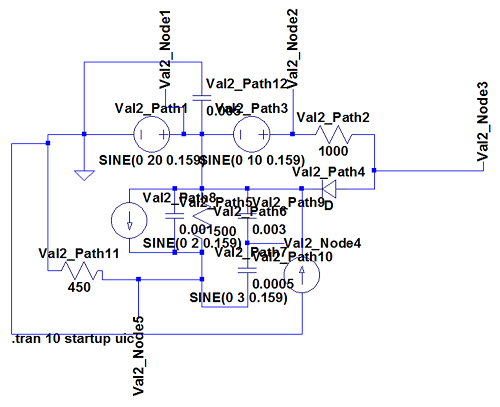
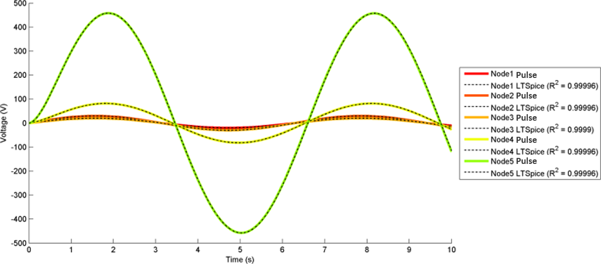
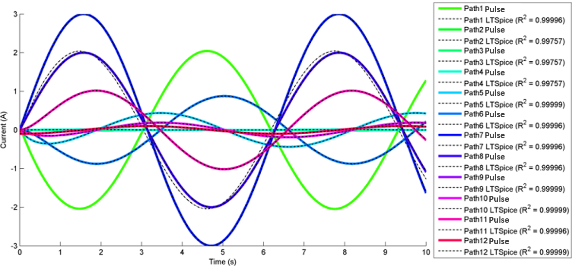
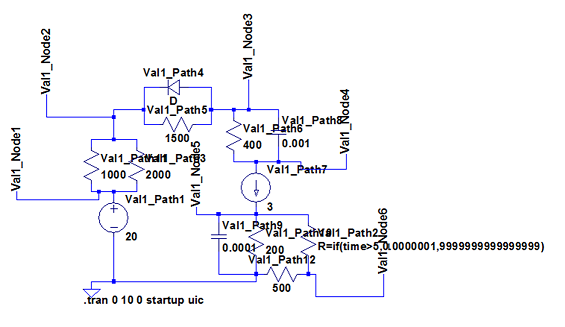
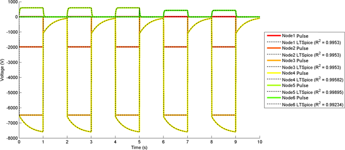
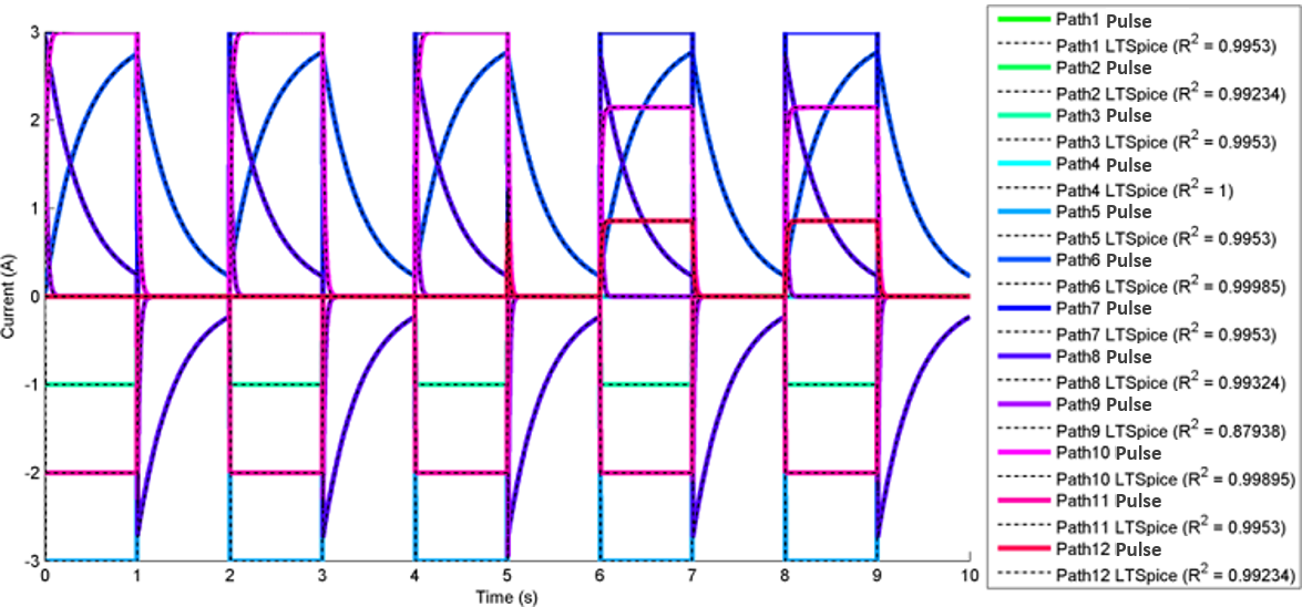
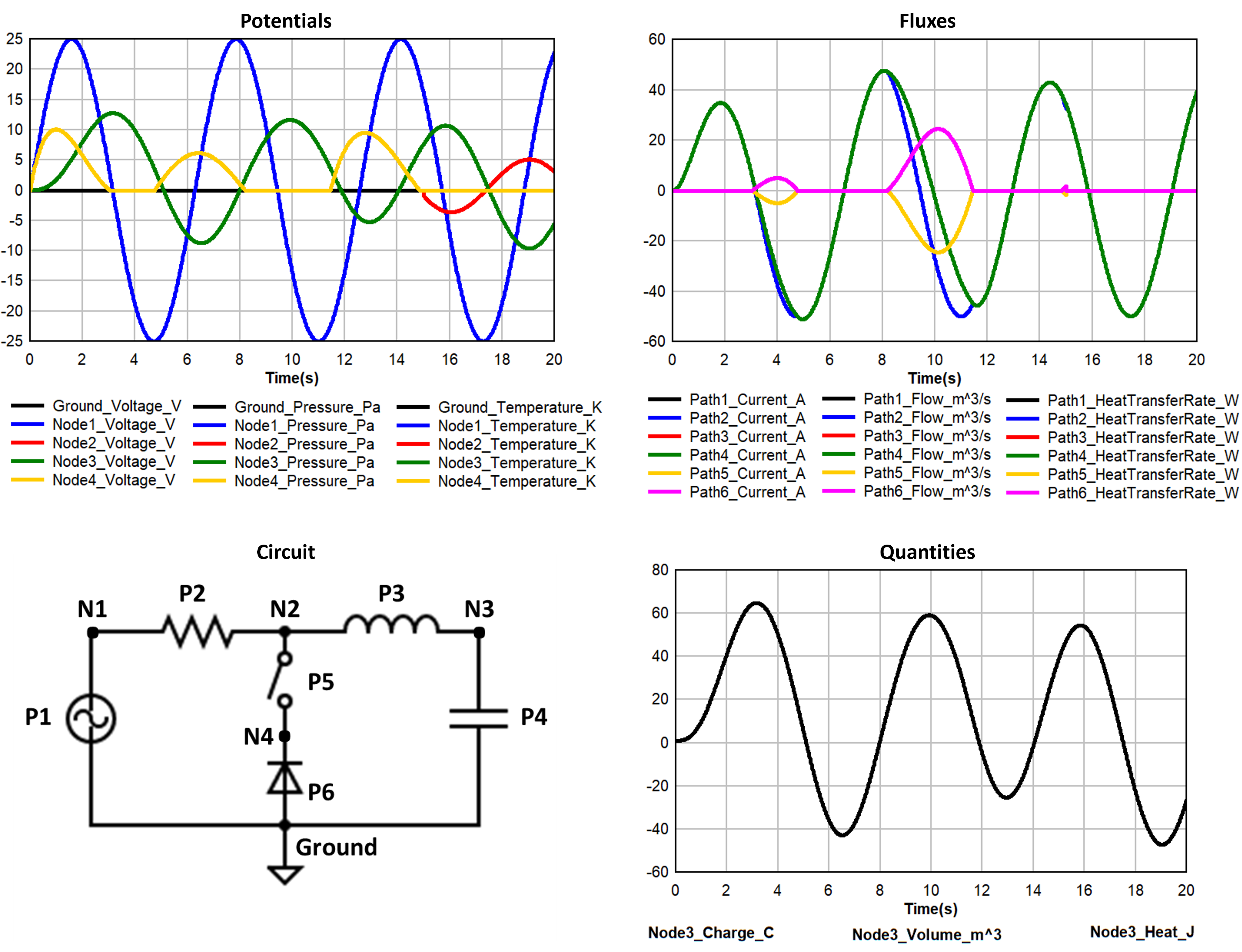
Figure 11 shows transient analysis results and the circuit diagram used for three sets of equivalent code blocks to illustrate the templated approach in setting up electrical, fluid, and thermal circuits.
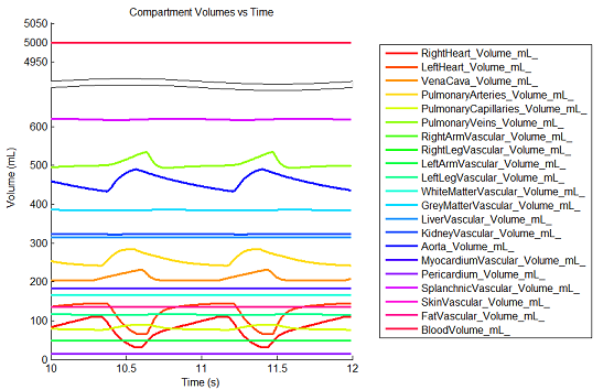
The engine has been shown to successfully conserve mass, energy, and momentum within all defined closed-loop systems. The successful conservation of mass provided by the solver is shown in Figure 12. The volume (quantity/charge) within cardiovascular circuit nodes through approximately 2.5 full heart beat cycles. The total volume of all compartments remains at a constant value of 5L throughout the entire process.
All basic Circuit Solver functionality is further validated and verified with specific unit tests that target individual methods. The following functionality has been successfully validated by individual tests:
- Incorrect usage errors
- Combined circuits
- Dynamically-changing elements
- Dynamically-changing circuits
- Added and removed elements
- Fluid, thermal, and electrical model types
- Non-zero reference node voltage
- Polarized elements
- Dynamically modifying capacitor charge
- Black boxes
Conclusion
The generalized circuit analysis techniques have successfully accomplished all of the goals for that area of the code. The solver implements the CDM effectively and generically in a way that allows for infinitely complex lumped parameter models that can also be combined. We made it simple to modify existing functionality and add new models. This has saved, and will continue to save, significant amounts of development time. The generic and modular design also allows for much easier bug finding and fixing, system parameter tuning, and system validation. The burden for the modeler is on creating a good model and not worrying about implementing sound physics math.
The Circuit Solver has also been designed such that it can be extracted from the enbgine and used for any software that needs to perform transient circuit analysis.
Future Work
Coming Soon
The list below includes some of the planned functionality additions.
- Functionality to create grey boxes for improved modularity between systems/subsystems and reduced processing speeds of interconnected circuits
Recommended Improvements
Other functionality that may be beneficial includes:
- A sensitivity analysis and error term determination
- An analysis of frequency constraints
- More circuit elements (i.e., amplifiers, transformers, transistors, non-ideal elements, zener diodes, etc.)
Appendices
Data Model Implementation
Glossary
CDM - Common Data Model
DC - Direct Current
GUI - Graphical User Interface
KCL - Kirkoff's Current Law
MNA - Modified Nodal Analysis
SPICE - Simulation Program with Integrated Circuit Emphasis