Overview
Abstract
The Renal system's purpose in the body is to filter blood. Each kidney is modeled in the engine using a single, lumped nephron to represent its behavior. By using this circuit analogue of a lumped nephron, the engine accurately simulates the major functions of the kidney: filtration, clearance, secretion, and reabsorption. Through these nephron-level processes, we are able to accurately recreate the mechanism by which urine is produced and blood is filtered. The renal system is complex and able to mechanistically and accurately recreate the clearance of the substances currently in the engine. The system passes the majority of validation and demonstrates the correct trends in scenarios that test specific functionality.
Introduction
Renal Physiology
The renal (or urinary) system's primary job is filtering the blood to remove waste and manage fluid volume, which helps the body maintain homeostasis.
Figure 1 shows the entire system and is labeled with the following:
- Urinary system
- Kidney
- Renal pelvis
- Ureter
- Urinary bladder
- Urethra (Left side with frontal section)
- Adrenal gland
- Renal artery and vein
- Inferior vena cava
- Abdominal aorta
- Common iliac artery and vein
- Liver
- Large intestine
- Pelvis
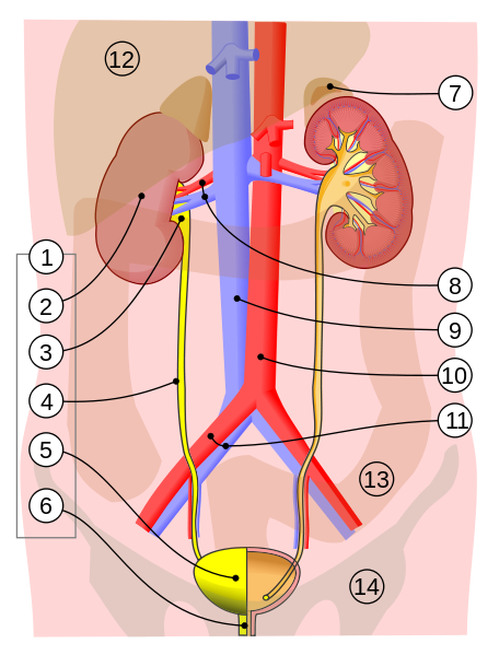 Figure 1 This is an illustration of the human renal system. The bounds of the system are generally accepted to be the combination of everything encompassing #1-6 (urinary system) and #8 renal artery and vein. [371]
After the blood enters the kidneys through the renal arteries, it is distributed into the nephrons through the branching afferent arteriole network. From the arterioles, the blood then travels into the glomerular capillaries. The capillary wall's permeability coupled with the pressure difference across the permeable layer allows filtration of about 20 percent [156] of the incoming blood into the Bowman's space and downstream into the tubules, vas rectum and, eventually, the collecting duct where the fluid travels through the ureters and into the bladder in the form of urine.
The average glomerular filtration rate (GFR) in a human is around 120 mL/min [381] between both kidneys. The filtered fluid primarily consists of the smaller particles in the blood, as a general rule less than 10 nm in diameter [381]. This filtered fluid will eventually become urine; however, most of the fluid will be reabsorbed back into the blood to preserve substance and fluid levels in the body. Some substances, such as creatinine, are not reabsorbed, making these good a clinical markers of GFR.
Pressure and GFR are tightly regulated through the tubuloglomerular feedback mechanism of the kidney. This mechanism allows for an increase or decrease in the diameter of the arteries on either side of the glomerular capillaries, effectively regulating down stream fluid flow and protecting the fragile capillaries of the glomerulus.
Once filtered, reabsorption and secretion both occur along the length of the tubules into the collecting ducts. In this area, the body reabsorbs many of the substances and, on average, over 99% of the water back into the blood [156]. Reabsorption is heavily dependent on the sodium concentration of the blood, the downstream pressure at the afferent arteriole, and osmotic and oncotic pressure gradients along the tubular cell walls and intra-vascular space. The kidneys influence the osmolarity of the urine by adjusting the amount of sodium and water excreted to the bladder. Secretion allows for further filtration of the blood by the kidneys via active transport of substances back into the tubules from the peritubular capillaries. All of these processes are tightly regulated and allow for careful management of substances levels within the entire body. Any water or substance that is not reabsorbed is moved to the bladder as urine through the collecting ducts.
By regulating the substance content of the blood, the kidneys are responsible for maintaining blood pH and nitrogen content over long periods of time. Nitrogen waste from the liver is excreted from the kidneys as urea, one of the primary constituents of urine. Bicarbonate is used by the blood as a buffer against much of the acidic content of the body. The kidneys are able to reabsorb virtually all of the filtered bicarbonate and even reclaim bicarbonate that has been used to buffer acids that are filtered into the renal tubules [381].
Renal Modeling
The Renal model lumps each kidney into a single nephron (Figure 2). The fluid flow through the kidney is modeled with an electrical circuit analogue, and the substance transport is a combination of the generic transporter and active filtration/reabsorption/secretion based on feedback and substance parameters. Alternatively, excretion can be directly applied and is governed via clearance equations - as with the drug model (Drugs Methodology). This is consistent with other system models, which also employ lumped parameter modeling.
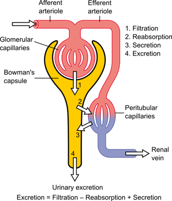 Figure 2 The basic anatomical structure of the nephron. The blood is filtered into the Bowman's capsule from the Glomerular Capillaries. Most of the fluid is then reabsorbed into Peritubluar Capillaries. The remaining fluid and substances continue through the tubules and are exreted into the bladder. [375]
 System Design
Background and Scope
Requirements
The Renal system needs to meet the following requirements in the engine:
- General kidney functions [152]
- Excretion of metabolic waste products and foreign chemicals
- Regulation of water and electrolyte balances
- Regulation of body fluid osmolality and electrolyte concentrations
- Regulation of arterial pressure
- Regulation of acid-base balance
- Secretion, metabolism, and excretion of hormones
- Gluconeogenesis
- Specific effects required by the Engine
- Nutritional states based on feeding, starvation, water loads, dehydration, and salt intake
- Renal stenosis and hypoperfusion
- General hematology: electrolytes, ions, blood gases, protein, urea, creatinine, hemoglobin, hematocrit, RBC, WBC, and Acid/Base Balance
- System parameters: Urine volume, osmolality, GFR, and BUN
- Respiratory acidosis/alkalosis, metabolic acidosis
- Drugs pharmacokinetics handling
- Extensible and flexible model
- Maintain conservation of mass and homeostasis
Previous Research
There have been numerous approaches to renal modeling in the past. The most significant results stem from a region-based modeling approach that discretizes the depth and allows varying permeability along the length of the nephron [213]. Focusing on the region encompassing the collecting duct allows for consideration of the flow in the tubules as well as interactions with the interstitial space. This space plays a key role in the re-absorption process and is modeled with striking detail. This model has been shown to be an extremely accurate representation of the urine concentrating mechanism along the length of the short and long nephron and has been shown to accurately model the two feedback mechanisms that control glomerular filtration and blood flow: the myogenic response and the tubuloglomerular feedback. This model uses a region-based approach to model a single collecting duct, then it scales results up to a system-wide representation. The idea of representing the kidney as a functional nephron is something that many other researchers in the past have used to accomplish very promising results regarding kidney functionality [250], [249], [351].
In each of these efforts the nephron is broken into its distinct sections and the reabsorption of substances and fluid is calculated at each point. Each calculation is done in series until the filtered fluid reaches the collecting ducts and exits as urine. By assuming the results carry over to the other nephrons in the kidney, these models are able to create realistic urine outputs under most conditions. While these models can show the tubular transport of substances and fluid in great detail, some do not directly show the renal hemodynamics at work to control glomerular pressure and GFR. In addition, many of these results are steady state rather than time-dependent, which limits the range of applications and outputs.
Many models use the Starling equation (Equation 1) to calculate the fluid flow between the tubules and blood. While this is generally considered to be an accurate representation of the fluid flow, this approach assumes a constant oncotic pressure. This makes the hydrostatic pressures the only dynamic inputs to the Starling equation. The accuracy of this approache can be enhanced by accounting for differences in the substance content in vascular compartments in the glomerular capillaries and deriving the respective oncotic pressures, which allows for a better representation of the pressure differential that drives the flow.
![\[{J_v} = {K_f}\left( {\left[ {{P_c} - {P_i}} \right] - \sigma \left[ {{\pi _c} - {\pi _i}} \right]} \right)\]](form_136.png)
Jv represents net fluid flow, Pc and Pi represent the capillary and interstitial hydrostatic pressures, πc and πi are the capillary and interstitial oncotic pressures, respectively, Kf is the filtration coefficient, and σ is the reflection coefficient. The equation uses a V=IR approach to derive the flow from the total pressure differential and the resistance, which is represented by the filtration and reflection coefficients.
There are other existing models that show the hemodynamics present within the kidney. The model shown by Moss [250] uses a network of nephrons and a fluid circuit to represent the kidney. The fluid circuit can affect the delivery of blood to the various glomerular capillaries by changing the resistance that represents the afferent arteriole. This allows the model to represent the physiological feedback from changes in sodium reabsorption, which can have notable effects on renal blood flow. The fidelity of this sort of model is very flexible, as it is entirely dependent on the detail put into the nephron. Unfortunately, as the complexity of the nephron model or the desired size of the network increases, it can become computationally intensive. This can cause problems when attempting to use this approach as part of a real-time model.
Approach
The Renal model includes both the upper and lower urinary tracts. The urine formation in the kidneys is simulated using a single lumped nephron model, which is the internal functional element shown as #2 in Figure 1. The computational representation of the system includes the renal artery that feeds into the afferent arteriole. Filtration takes place through the glomerular capillaries, and re-absorption occurs through the tubules into the peritubular capillaries. The peritubular capillaries connect into the vena cava, allowing transport back into the cardiovascular system. The ureter and bladder make up the rest of the kidney model in the engine. This model of the renal system allows for tubuloglomerular feedback and re-absorption feedback. These mechanisms allow for diuresis under heavy pressure loads and filtrate regulation under variable pressure scenarios.
The Renal fluid circuit is inserted in the the circulatory system and replaces a calibrated three-element (two resistances and one compliance) Windkessel model that is used for Cardiovascular validation. In this way, the standalone circuit at a resting physiologic state matches from a total fluid mechanics standpoint.
The transport of substances is a combination of the generic methodology and active filtration at specific locations. However, if a substance has a defined renal clearance parameter, as with drugs, that value is directly applied and is only dependent on blood flow changes.
Data Flow
The Renal System determines its state at every time step through a three-step process: Preprocess, Process, and Postprocess. In general, Preprocess sets the circuit element values based on feedback mechanisms and engine settings/actions. Process uses the generic circuit calculator to compute the entire state of the circuit. Postprocess is used to advance time. More specifics about these steps are detailed below.
Reset, Conditions, and Initialization
During initialization of the system, the filterability parameter for each defined substance is calculated. This is only done and set once because it is only dependent on the substance's molecular weight and charge in blood, which do not change.
The two Renal system conditions are also applied using the engine stabilization methodology. Renal stenosis and consume meal are discussed in detail later.
Preprocess
Preprocess is called by the engine to apply the system-specific feedback mechanisms. Each of these mechanisms for the Renal system are described individually and in detail later.
Process
The generic circuit solving and transporting are done on the combined circulatory system inside the Cardiovascular system. After the new state of the circuit is determined, active transport is performed, and the system data is calculated and set.
Post Process
The Postprocess step moves values calculated in the Process step from the next time step calculation to the current time step calculation. The current implementation has no specific postprocess functionality for the Renal system. All postprocessing is done on the combined circulatory system inside the Cardiovascular system.
Assessments
There is one assessment that is done within the Renal system - urinalysis. This is a data call that requires further calculations and analysis to create outputs. It is discussed in detail later.
Features, Capabilities, and Dependencies
Circuit
The Renal circuit (Figure 3) determines blood and urine pressure, flow, and volume, organized by compartments. These compartments are comprised of lumped parameter models that use resistors, capacitors, pressure sources, and valves. The number of lumped parameter models used to represent the Renal System was chosen to provide a level of fidelity that meets the requirements of the overall project and to provide sufficient system capability.
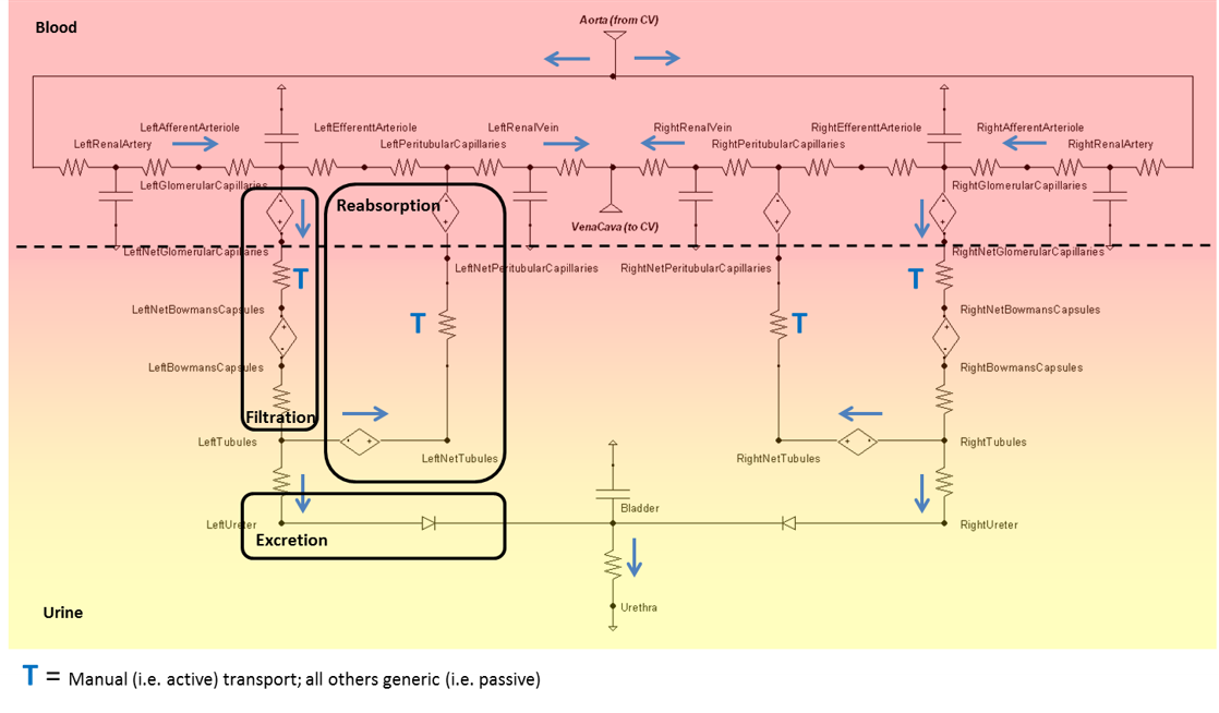
Nodes serve as the connection points for paths and are the locations at which pressures are measured. Each Renal node contains a pressure value, which is given with respect to the atmospheric reference node (indicated in the diagram by the equipotential symbol). Nodes can also hold the values for volume or the mass and concentration of substances. Paths contain information about the flow (volume per time) and volumes of compliances. The Circuit Methodology document contains more information about circuit definitions and modeling. The Substance Transport Methodology contains more information about the substance transport and mass and concentration calculations.
Dynamic pressure sources are used at the filtration and reabsorption locations to model the colloid osmotic pressures caused by protein in the fluid. These pressures, in combination with the hydrostatic pressures, give a correct total pressure difference to cause a correct net fluid flow.
The bladder is currently modeled as a constant pressure source and the volume is calculated directly based on the flow through that source. Future versions will likely replace the source with a compliance and incorporate a peristaltic flow model.
The compliance and volume of the Renal circuit are determined by validated volume data and model assumptions made regarding the various nodes in the renal system. These compliances allow for some volume variability as the capillaries experience pressure and flow changes.
The volume distribution of the Renal system is as follows:
- Kidneys = 69.6 mL
- Right Kidney = 34.8 mL
- Right Small Vasculature = 17.4 mL
- Right Glomerular Capillary (compliance) = 3.48 mL
- Right Peritubular Capillary = 3.48 mL
- Right Efferent Arteriole = 3.48 mL
- Right Bowmans Capsule = 3.48
- Right Afferent Arteriole = 3.48 mL
- Right Large Vasculature = 17.4 mL
- Right Renal Vein (compliance) = 5.8 mL
- Right Renal Artery (compliance) = 5.8 mL
- Right Tubules = 5.8
- Right Small Vasculature = 17.4 mL
- Left Kidney = 34.8 mL
- Left Small Vasculature = 17.4 mL
- Left Glomerular Capillary (compliance) = 3.48 mL
- Left Peritubular Capillary = 3.48 mL
- Left Efferent Arteriole = 3.48 mL
- Left Bowmans Capsule = 3.48
- Left Afferent Arteriole = 3.48 mL
- Left Large Vasculature = 17.4 mL
- Left Renal Vein (compliance) = 5.8 mL
- Left Renal Artery (compliance) = 5.8 mL
- Left Tubules = 5.8
- Left Small Vasculature = 17.4 mL
- Right Kidney = 34.8 mL
The Renal circuit contains 11 resistances for each kidney, and a shared urethra resistance - see Figure 4. The urethra (number 12) is typically set as an open switch (approximately infinite resistance), unless the patient is urinating, when it becomes closed to allow flow out of the bladder.
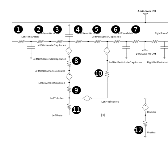 Figure 4 The resistances in the left kidney are numbered for further description.
Baseline resistances were determined by leveraging reference pressure and flow values from literature. Each resistance is calculated using Equation 2, where R is the resistance along the path, ΔP is the pressure difference between the source and target nodes, and F is the fluid flow through the path.
![\[R = \frac{{\Delta P}}{F}\]](form_137.png)
The untuned baseline resistance values were calculated using the values in Table 1. These values and the model were verified with unit testing using a static arteriole pressure equal to the normal mean value.
| Location | Number in Figure | Beginning Pressure (mmHg) | Ending Pressure (mmHg) | Flow (mL/min) | Resulting Baseline Resistance (mmHg/mL/min) |
|---|---|---|---|---|---|
| Arteries | 1 | 100 | 100 | 600 | 0.0 |
| RenalArteries | 2 | 100 | 85 | 600 | 0.0250 |
| AfferentArteriole | 3 | 85 | 60 | 600 | 0.0417 |
| GlomerularCapillaries | 4 | 60 | 59 | 537.5 | 0.0019 |
| EfferentArteriole | 5 | 59 | 18 | 537.5 | 0.0763 |
| PeritubularCapillaries | 6 | 18 | 8 | 600 | 0.0167 |
| RenalVeins | 7 | 8 | 4 | 600 | 0.0066 |
| GlomerularFilter | 8 | 28 | 18 | 62.5 | 0.1600 |
| Tubules | 9 | 18 | 6 | 62.5 | 0.1920 |
| Reabsorption | 10 | -9 | -19 | 62 | 0.1613 |
| Ureter | 11 | 6 | 4 | 0.52 | 3.846 |
| Urethra (during urination) | 12 | 4 | 0 | 1320 | 0.0030 |
Patient Variability
The total vascular volume of the renal system in is defined to be a fraction of the body total, making kidney volume directly dependent upon the patient data: height, weight, and gender. The volume fraction of both kidneys is set to be 0.0202, or about 1/50th of total blood volume [381]. This volume is then divided in half to populate the total vascular volume of one kidney. For a further breakdown of the volume of each kidney compartment see Features.
Feedback
Colloid Osmotic Pressure
The net filtration and reabsorption pressures are determined by the sum of the hydrostatic and colloid osmotic forces across the membranes. While the hydrostatic pressure is automatically handled using the generic circuit algorithms, the colloid osmotic pressure needs to be determined specifically. This is done by using the Landis-Pappenheimer equation (Equation 4) that is dependent on total protein [192]. Since the engine tracks albumin, a constant relationship between total protein and albumin can be leveraged using Equation 3. *CTP* is the local concentration of total protein, *CA* is the local concentration of albmuin, and *PCO* is colloid osmotic pressure.
![\[{C_{TP}} = 1.6{C_A}\]](form_138.png)
![\[{P_{CO}} = 2.1{C_{TP}} + 0.16C_{_{TP}}^2 + 0.009C_{_{TP}}^3\]](form_139.png)
The Landis-Pappenheimer equation is applied at the pressure sources numbered in Figure 5.
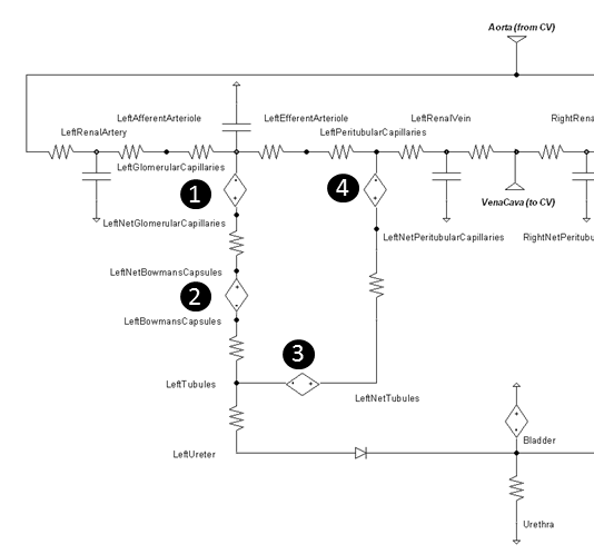 Figure 5 The four pressure sources that represent the colloid osmotic pressure are determined via the local albumin concentration.
Table 2 gives the typical colloid osmotic pressure values. The tubular osmotic pressure is set constant in our model and does not change because we are not modeling the interstitial space. The remaining osmotic pressures will increase and decrease in relation to the local albumin concentration variations. See Table 5 for resulting values when albumin concentration feedback is applied.
| Location | Number in Figure | Baseline Colloid Osmotic Pressure (mmHg) |
|---|---|---|
| GlomerularCapillariesOsmoticPressure | 1 | -32 |
| BowmansCapsulesOsmoticPressure | 2 | 0 |
| TubulesOsmoticPressure | 3 | -15 |
| PeritubularCapillariesOsmoticPressure | 4 | -32 |
Fluid Permeability
The hydraulic and colloid osmotic pressure gradients across the glomerular and pertitubular capillary membranes cause the movement of fluid. The rate of fluid movement is a function of the fluid permeability of the membranes, the total membrane surface area, and the pressure gradient. Considering a nominal pressure that is equal to the linear integral of the effective pressure over the length of the glomerular capillary (with the effective pressure being the difference between the hydrostatic and colloid osmotic pressure gradients at each point along the length of the capillary), the glomerular filtration rate is proportional to the nominal pressure, as shown in Equation 5.
![\[GFR = {L_p}{S_f}\int {\left[ {\left( {{P_g}\left( x \right) - {P_B}} \right) - \sigma \left( {{\pi _g}\left( x \right) - {\pi _B}} \right)} \right]dx} = {L_p}{S_f}\Delta P\]](form_140.png)
Lp is the hydraulic conductivity of the membrane and Sf is the surface area. Relating the equation above to the linear fluid dynamics equations, it is apparent that the resistance to flow can be modeled as 1/(Lp Sf). The product, Lp Sf, has been called the glomerular filtration coefficient [367]. A similar reabsorption coefficient can be derived from the equations governing the reabsorption of water in the renal tubules [367].
The hydraulic permeability is computed for use in the model using filtration coefficients reported in literature as well as surface area estimates. The surface area of the glomerular capillaries is estimated to be about 2.0 square meters per human kidney [379]. The surface area of the peritubular capillaries is larger than the glomerular capillaries [367]. However, how much larger is difficult to quantify. For the model, it is assumed that the surface area of the peritubular capillaries is 25 percent larger than the surface area of the glomerular capillaries. Using the glomerular filtration coefficient value of 13 mL/min-mmHg for both kidneys as reported in [367] (6.5 mL/min-mmHg each kidney assuming an equal distribution of surface area), the hydraulic conductivity of the glomerular capillaries is calculated to be 3.67647 mL/m2-min-mmHg. Likewise, using the reabsorption coefficient value of 10 mL/min-mmHg for both kidneys [367], the hydraulic conductivity of the peritubular capillaries is computed to be 2.91747 mL/m2-min-mmHg.
These values are applied in the model as the resistances circled in Figure 6 and are determined using Equation 6. RFilt is the membrane fluid resistance, kp is the permeability, and A is the total membrane area.
![\[{R_{filt}} = \frac{1}{{{k_p}A}}\]](form_141.png)
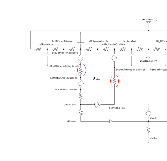 Figure 6 The membrane fluid filtration for both glomerular filtration and peritubular reabsorption locations are modeled as the resistances circled in red.
Ultrafiltration
Individual substance transport from the glomerular capillaries to the bowmans capsules is directly proportional to the fluid glomerular filtration rate and filterability value based on molecular size and charge. The glomerular capillary membrane is thicker than most other capillaries, but it is also much more porous and filters fluid at a high rate [152]. Ultrafiltration is a largely passive mechanism.
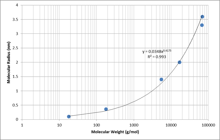
Empirical data was used to determine a generic relationship between molecular weight and molecular radius. Values for water, glucose, inulin, myoglobin, hemoglobin, and albumin were used to determine the best fit shown in Figure 7 [304].
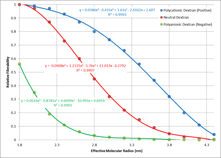
Electrical charge of each molecule has an effect on the total filterability. A negative charge restricts filtration, where as a positive charge filters more readily. Figure 8 shows the relative filterability best fit for positively charged, neutral, and negatively charged molecules as a function of molecular radius (determined using the relationship in Figure 7).
Reabsorption
Reabsorption works in much the same way as glomerular filtration, with additional active mechanisms that are different for each substance. For the Renal model, all of the active transport mechanisms are lumped into a single reabsorption ratio parameter defined for each substance. This ratio represents the extent to which the substance is reabsorbed from the tubules to the peritubular capillaries in relation to the fluid flow. Therefore, a value of 1.0 indicates that the substance is reabsorbed at the same rate as water, values below 1.0 indicate that it is reabsorbed more avidly than water, and values above 1.0 indicate that it is reabsorbed less avidly than water. Each substance also has a transport maximum value defined that prevents substance mass movement at a specific transient value. A value of infinity is allowed for both reabsorption-specific substance parameters.
Reabsorption Feedback
Pressure natriuresis and diuresis are simulated in the Renal model through reabsorption premeability modifiers. In the kidneys, as arterial pressure increases, shear stresses are developed along the cell walls. These stresses induce the release of nitric oxide, which is diffused downstream to the tubules of the nephron. This serves to decrease the sodium reabsorption rate through select entry pathways [259]. This decrease in sodium resabsorptioin decreases the osmotic gradient along this fluid path, consequently leading to a coupled decrease in fluid reabsorption. The engine does not currently support nitric oxide, so we model this mechanism by coupling the fluid permeability characteristics of the tubules as function of arterial pressure. This allows for the connection to downstream pressure changes and sodium/water reabsorption. A second order polynomial (See Equation 7) is fit to the data taken from [152] that scales the tubules' fluid permeability as a function of arterial pressure. This permeability then directly affects the resistance along the reabsorption pathway, leading to a decrease or increase in water/sodium transport. Diruetic administration can also inhibit the reabsorption by modifying the tubular lumen permeabilty as a function of plasma concentration of Furosemide, Drugs Methodology.
![\[{k_p} = \left( {2.01 \times {{10}^{ - 6}}} \right)P_A^2 - \left( {8.1 \times {{10}^{ - 4}}} \right)P_A^{} + 9.4 \times {10^{ - 2}}\]](form_142.png)
Diuretic Response
In addition to alterations in permeability due to ion concentration and perfusion pressure, the renal system's reabsorption pathway can also be effected by diuretic concentrations in the blood plasma. These concentrations directly effect the tubular permeability, simulating Furosmide binding to the Na-K-2Cl symporter. This effect is accounted for by calculating the response due to plasma concentrations in the Drug methodology. This permeability modifier is then stored and accessed in the Renal system each time step to calculate the reabsorption pathway resistance:
![\[{k_p}_{i+1} = {k_p}_i * K_{mod}(C_p) \]](form_143.png)
Here Kmod(Cp) is the modification coefficient calculated as a hill type functional response to Furosemide blood plasma concentration, Cp.
Secretion
Flow of substances can be directed from the peritubular capillaries into the tubules through secretion. As fluid travels along the tubules and into the collecting ducts of the nephron, various stages of the journey either reabsorb or secret substances and water back into and out of the fluid. One of the most important tasks of the renal system is handling of potassium levels in the blood stream. Secretion is one of the main ways that the renal system handles this task with active transport mechanisms located along the tubular cell wall. The engine simulates this active handling of potassium by allowing for secretion into the ureter from peritubular capillaries. Mass is calculated and tightly regulated by the renal system by actively moving any mass above a certain threshold directly into the urine. The engine does not currently support disturbances to the permeable layer and so shifts in potassium levels in the body will not currently be possible.
Bladder and Excretion
Excretion of fluid and substances to the bladder is done generically by the circuit solver (Circuit Methodology) and transporter (Substance Transport Methodology).
Tubuloglomerular Feedback
One of the main mechanisms for kidney regulation of renal blood flow due to changes in the mean arterial pressure is tubuloglomerular feedback. This is caused by a transient increase in GFR that leads to an increased sodium delivery to the macula densa [304]. For the Renal model, the macula densa is lumped with all tubules. When the mass flow rate of sodium changes in the tubules, a response is applied.
Within an autoregulatory range of 80 to 180 mmHg for the MAP, the renal blood flow is is maintained by either constricting (increased resistance) or dilating (decreased resistance) the afferent areteriole [304]. A higher sodium mass flow rate in the tubules leads to a higher resistance, and a lower mass flow rate leads to a lower resistance (see Figure 10). The minimum and maximum resistances for the afferent arteriole were determined through a unit test to be 1.7 mmHg/mL-s (at MAP of 80 mmHg) and 12.382 mmHg/mL-s (at MAP of 180 mmHg).
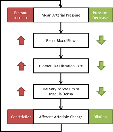 Figure 10 A flow diagram showing the tubuloglomerular response to increased and decreased MAP. [304]
High frequency oscillations of the tubuloglomerular feedback are damped using the tuning constant, alpha, in Equation 8. *RAff* is the afferent arteriole resistance where i and i+1 signify the current and the next resistance respectively, ||Δ UNa|| is the normalized change in sodium flow into the tubules. Normalization is used to decrease sensitivity of the response. Large fluctuations are not only physiologically incorrect but also create instabilities during heartbeats. The sodium mass flow setpoint is the expected value with a stable standard patient. Figure 12 indicates good agreement between the mechanics of the engine and experimental data. Autoregulation is handled entirely from the TGF response, with the myogenic response not modeled currently.
![\[R_{Aff}^{i + 1} * = \frac{{R_{Aff}^i}}{{R_{Aff}^{i + 1}}} + \alpha \left\| {\Delta {U_{Na}}} \right\|\]](form_144.png)
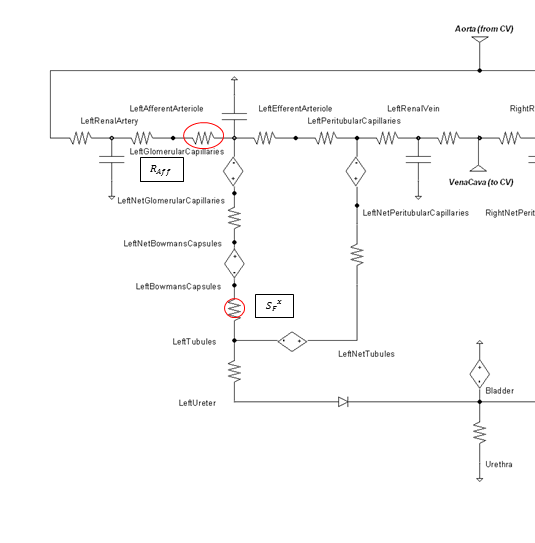 Figure 11 The circle shows the location used to determine the sodium value, and the resistance where the feedback is applied is denoted with an oval.
 |  |
Osmoreceptor Feedback
When osmolarity (plasma sodium concentration) increases/decreases above/below normal the osmoreceptor feedback system compensates in the way shown in Figure 13. Increased water permeability in the distal nephron segments causes increased water reabsorption and excretion of a small volume of concentrated urine [152]. This mechanism tends to keep the plasma sodium concentration stable and was calibrated with extended multi-hour simulations.
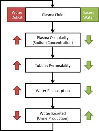 Figure 13 A flow diagram showing the osmoreceptor response to increased and decreased plasma sodium concentration. [152]
The sensitivity of the osmoreceptor feedback is calibrated using the tuning constant x in Equation 9. kP is the reabsorption fluid permeability, CSP is the sodium plasma concentration in the tubules, and CSP,Set is the setpoint. The sodium plasma concentration setpoint is the expected value with a stable standard patient.
![\[{k_p} * = {\left( {\frac{{{C_{SP}}}}{{{C_{SP,Set}}}}} \right)^x}\]](form_145.png)
Gluconeogenesis
Gluconeogenesis is a metabolic pathway that results in the generation of glucose from non-carbohydrate carbon substrates, such as lactate. Within the Renal system, this process is applied by converting excreted lactate at a one-to-one mass ratio into reabsorbed glucose. This effectively removes all lactate from the urine until the transport maximum is achieved. If the converted mass exceeds the transport maximum, it is capped and the remainder continues to the urine.
Renal Clearance
Some substance in the engine specify a single renal clearance parameter (e.g. drugs) instead of inputs required for the previously described active transport mechanisms. If so, that value is directly applied and is only dependent on blood flow and plasma concentration changes. Details on this behavior are in Drugs Methodology.
Dependencies
The Renal system is directly connected to the Cardiovascular system at the aorta and vena cava. The boundary condition feedback in and out is automatically handled through the node and path interactions. It also shares a reference node.
Assumptions and Limitations
There are several assumptions that were used in creating this Renal model:
- All nephrons in each kidney are lumped together
- Secretion effects are lumped with reabsorption
- No specific substance metabolism is modeled
- Both kidneys are identical
- The difference between blood and urine is substance dependent only; they are the same fluid from a physics standpoint
Conditions
Consume Meal
The consume meal condition takes the resting renal clearance of each substance and extrapolates how much would be removed during a specified fasting period. The substances are then decremented accordingly. The loss of fluid is handled by the Energy system (Energy Methodology). In this way, both dehydration and starvation can be modeled. See the Gastrointestinal Methodology document for more information.
Actions
Urinate
Urination empties the bladder. This can be called as an action or will automatically occur with the functional incontinence event. This action decreases the urethra resistance to allow the bladder to empty to 1 mL. The fluid mechanics and transport are done generically by the circuit solver and transporter respectively.
Events
Diuresis
Diuresis is the state of producing urine at a significantly faster rate than normal. In the engine, we consider diuresis to occur when the average production rate of urine exceeds 8 mL/min [369], and the event is reversed when the average production rate of urine falls below 7.5 mL/min.
Antidiuresis
Antidiuresis occurs when small quantities of urine are being produced at an osmolarity greater than that of the plasma. For the engine, this event is thrown when the average urine production rate is less than 0.5 mL/min and the urine osmolarity is greater than 280 mOsm/L [381]. The event is reversed when either the urine production rate rises above 0.55 mL/min or the urine osmolarity falls below 275 mOsm/L.
Natriuresis
Natriuresis is the state of an unusually high rate of sodium excretion into the urine. In the engine, the setpoint for natriuresis is an average sodium excretion rate of 14.4 mg/min, or 6 times the resting sodium excretion rate [249]. The event is reversed when the average sodium excretion rate falls below 14.0 mg/min.
Functional Incontinence
Functional incontinence occurs when the bladder becomes too full of urine and automatially urinates. When the urine volume exceeds the maximum volume of the bladder in the engine, 400 mL, the functional incontinence event is thrown and a urinate action is automatically executed.
Assessments
Urinalysis
Validation of the urine panel is done by analyzing at the resting physiologic quantities. Urine color is determined based on the osmolality of the urine according to Table 3 below. Urine blood content registers as positive if the concentration of hemoglobin in the urine is greater than 0.15 ug/mL [390]. Currently, the presence of blood does not affect the color of the urine, with urine color being determined entirely by osmolality of the urine, Table 3.
| Urine Osmolality | Urine Color |
|---|---|
| UrineOsmolality <= 400 mOsm/kg | Pale Yellow |
| 400 < UrineOsmolality <=750 mOsm/kg | Yellow |
| UrineOsmolality > 750 mOsm/kg | Light Brown |
Standard Male
| Property Name | Expected Value | Engine Value | Percent Error | Notes |
|---|---|---|---|---|
| SpecificGravity | [1.00, 1.04] [381] [390] | Mean of 1.04 | 0.00% |
Standard Female
| Property Name | Expected Value | Engine Value | Percent Error | Notes |
|---|---|---|---|---|
| SpecificGravity | [1.00, 1.04] [381] [390] | Mean of 1.04 | 0.00% |
Results and Conclusions
Validation - Resting Physiologic State
Validation results for system and compartment quantities for a resting standard patient are listed in Table 5 and Table 6. System-level quantities show favorable agreement with validation values. The pressure value discrepancies in urine compartments can be largely explained by the Renal model's lack of a specific extracellular space that affects both the hydrostatic and osmotic pressures.
Standard Male
| Property Name | Expected Value | Engine Value | Percent Error | Notes |
|---|---|---|---|---|
| FiltrationFraction | 0.20 [152] | Mean of 0.18 | 10.1% | GFR/RenalPlasmaFlow |
| GlomerularFiltrationRate(L/day) | 180.0 [152] | Mean of 147.5 | 18.1% | |
| RenalBloodFlow(mL/min) | 1064.0 [379] | Mean of 1049.1 | 1.40% | |
| RenalPlasmaFlow(mL/min) | 638.4 [381] | Mean of 562.1 | 12.0% | Dependent on Hematocrit |
| RenalVascularResistance(mmHg_min/mL) | 0.080 [152] | Mean of 0.086 | 8.07% | |
| UrineOsmolality(mOsm/kg) | [50, 1200] [381] | Mean of 630 | 0.00% | |
| UrineOsmolarity(mOsm/L) | [50, 1200] [381] | Mean of 649 | 0.00% | |
| UrineProductionRate(L/day) | 1.50 [152] | Mean of 1.32 | 11.8% | |
| UrineSpecificGravity | [1.003, 1.040] [381] [390] | Mean of 1.037 | 0.00% | |
| UrineUreaNitrogenConcentration(g/L) | [5.0, 10.0] [381] | Mean of 8.6 | 0.00% | |
| LeftAfferentArterioleResistance(mmHg_min/mL) | 0.042 [152] | Mean of 0.042 | 1.60% | (85mmHg - 60mmHg) / (RenalBloodFlow / 2) |
| LeftBowmansCapsulesHydrostaticPressure(mmHg) | 18.0 [152] | Mean of 20.8 | 15.7% | |
| LeftBowmansCapsulesOsmoticPressure(mmHg) | 0.00 [152] | Mean of 0.00 | 0.00% | |
| LeftEfferentArterioleResistance(mmHg_min/mL) | 0.076 [152] | Mean of 0.077 | 1.46% | (59mmHg - 18mmHg) / ((RenalBloodFlow - GFR) / 2) |
| LeftFiltrationFraction | 0.20 [152] | Mean of 0.18 | 10.1% | GFR/RenalPlasmaFlow |
| LeftGlomerularCapillariesHydrostaticPressure(mmHg) | 60.0 [152] | Mean of 59.8 | 0.349% | |
| LeftGlomerularCapillariesOsmoticPressure(mmHg) | -32.0 [152] | Mean of -32.0 | 0.00% | |
| LeftGlomerularFiltrationCoefficient(mL/min_mmHg) | 12.5 [152] | Mean of 7.4 | 40.8% | Rate/NetPressure |
| LeftGlomerularFiltrationRate(L/day) | 90.0 [152] | Mean of 73.7 | 18.1% | Total GFR / 2 |
| LeftGlomerularFiltrationSurfaceArea(cm^2) | [7250, 23250] | Mean of 20000 | 0.00% | 5000-15000 cm^2 per 100 g renal tissue [381] mass of 2 kidneys in adult male = 310 g / 2 [379] |
| LeftNetFiltrationPressure(mmHg) | 10.0 [152] | Mean of 7.0 | 30.4% | |
| LeftNetReabsorptionPressure(mmHg) | 10.0 [152] | Mean of 7.7 | 22.7% | |
| LeftPeritubularCapillariesHydrostaticPressure(mmHg) | 13.0 [152] | Mean of 22.2 | 71.0% | |
| LeftPeritubularCapillariesOsmoticPressure(mmHg) | -32.0 [152] | Mean of -32.0 | 0.00% | |
| LeftReabsorptionFiltrationCoefficient(mL/min_mmHg) | 6.2 [152] | Mean of 6.6 | 6.00% | Rate/NetPressure |
| LeftReabsorptionRate(mL/min) | 62.0 [152] | Mean of 50.7 | 18.2% | TotalReabsorptionRate/2 |
| LeftTubularOsmoticPressure(mmHg) | -15.0 [152] | Mean of -15.0 | 0.00% | |
| RightAfferentArterioleResistance(mmHg_min/mL) | 0.042 [152] | Mean of 0.042 | 1.60% | (85mmHg - 60mmHg) / (RenalBloodFlow / 2) |
| RightBowmansCapsulesHydrostaticPressure(mmHg) | 18.0 [152] | Mean of 20.8 | 15.7% | |
| RightBowmansCapsulesOsmoticPressure(mmHg) | 0.00 [152] | Mean of 0.00 | 0.00% | |
| RightEfferentArterioleResistance(mmHg_min/mL) | 0.076 [152] | Mean of 0.077 | 1.46% | (59mmHg - 18mmHg) / ((RenalBloodFlow - GFR) / 2) |
| RightFiltrationFraction | 0.20 [152] | Mean of 0.18 | 10.1% | GFR/RenalPlasmaFlow |
| RightGlomerularCapillariesHydrostaticPressure(mmHg) | 60.0 [152] | Mean of 59.8 | 0.349% | |
| RightGlomerularCapillariesOsmoticPressure(mmHg) | -32.0 [152] | Mean of -32.0 | 0.00% | |
| RightGlomerularFiltrationCoefficient(mL/min_mmHg) | 6.2 [152] | Mean of 7.4 | 18.4% | Rate/NetPressure |
| RightGlomerularFiltrationRate(L/day) | 90.0 [152] | Mean of 73.7 | 18.1% | Total GFR / 2 |
| RightGlomerularFiltrationSurfaceArea(cm^2) | [7250, 23250] | Mean of 20000 | 0.00% | 5000-15000 cm^2 per 100 g renal tissue [381] mass of 2 kidneys in adult male = 310 g / 2 [379] |
| RightNetFiltrationPressure(mmHg) | 10.0 [152] | Mean of 7.0 | 30.4% | |
| RightNetReabsorptionPressure(mmHg) | 10.0 [152] | Mean of 7.7 | 22.7% | |
| RightPeritubularCapillariesHydrostaticPressure(mmHg) | 13.0 [152] | Mean of 22.2 | 71.0% | |
| RightPeritubularCapillariesOsmoticPressure(mmHg) | -32.0 [152] | Mean of -32.0 | 0.00% | |
| RightReabsorptionFiltrationCoefficient(mL/min_mmHg) | 6.2 [152] | Mean of 6.6 | 6.00% | Rate/NetPressure |
| RightReabsorptionRate(mL/min) | 62.0 [152] | Mean of 50.7 | 18.2% | TotalReabsorptionRate/2 |
| RightTubularOsmoticPressure(mmHg) | -15.0 [152] | Mean of -15.0 | 0.00% |
Standard Female
| Property Name | Expected Value | Engine Value | Percent Error | Notes |
|---|---|---|---|---|
| FiltrationFraction | 0.20 [152] | Mean of 0.15 | 24.9% | GFR/RenalPlasmaFlow |
| GlomerularFiltrationRate(L/day) | 180.0 [152] | Mean of 112.2 | 37.7% | |
| RenalBloodFlow(mL/min) | 833.0 [379] | Mean of 896.6 | 7.64% | |
| RenalPlasmaFlow(mL/min) | 499.8 [381] | Mean of 508.0 | 1.64% | Dependent on Hematocrit |
| RenalVascularResistance(mmHg_min/mL) | 0.080 [152] | Mean of 0.101 | 26.2% | |
| UrineOsmolality(mOsm/kg) | [50, 1200] [381] | Mean of 646 | 0.00% | |
| UrineOsmolarity(mOsm/L) | [50, 1200] [381] | Mean of 666 | 0.00% | |
| UrineProductionRate(L/day) | 1.50 [152] | Mean of 0.67 | 55.3% | |
| UrineSpecificGravity | [1.003, 1.040] [381] [390] | Mean of 1.037 | 0.00% | |
| UrineUreaNitrogenConcentration(g/L) | [5.0, 10.0] [381] | Mean of 9.2 | 0.00% | |
| LeftAfferentArterioleResistance(mmHg_min/mL) | 0.042 [152] | Mean of 0.042 | 0.531% | (85mmHg - 60mmHg) / (RenalBloodFlow / 2) |
| LeftBowmansCapsulesHydrostaticPressure(mmHg) | 18.0 [152] | Mean of 14.4 | 20.2% | |
| LeftBowmansCapsulesOsmoticPressure(mmHg) | 0.00 [152] | Mean of 0.00 | 0.00% | |
| LeftEfferentArterioleResistance(mmHg_min/mL) | 0.076 [152] | Mean of 0.077 | 0.274% | (59mmHg - 18mmHg) / ((RenalBloodFlow - GFR) / 2) |
| LeftFiltrationFraction | 0.20 [152] | Mean of 0.15 | 24.6% | GFR/RenalPlasmaFlow |
| LeftGlomerularCapillariesHydrostaticPressure(mmHg) | 60.0 [152] | Mean of 51.7 | 13.9% | |
| LeftGlomerularCapillariesOsmoticPressure(mmHg) | -32.0 [152] | Mean of -32.0 | 0.00% | |
| LeftGlomerularFiltrationCoefficient(mL/min_mmHg) | 12.5 [152] | Mean of 7.4 | 40.8% | Rate/NetPressure |
| LeftGlomerularFiltrationRate(L/day) | 90.0 [152] | Mean of 56.1 | 37.7% | Total GFR / 2 |
| LeftGlomerularFiltrationSurfaceArea(cm^2) | [7250, 23250] | Mean of 20000 | 0.00% | 5000-15000 cm^2 per 100 g renal tissue [381] mass of 2 kidneys in adult male = 310 g / 2 [379] |
| LeftNetFiltrationPressure(mmHg) | 10.0 [152] | Mean of 5.3 | 47.0% | |
| LeftNetReabsorptionPressure(mmHg) | 10.0 [152] | Mean of 5.8 | 41.8% | |
| LeftPeritubularCapillariesHydrostaticPressure(mmHg) | 13.0 [152] | Mean of 19.6 | 50.4% | |
| LeftPeritubularCapillariesOsmoticPressure(mmHg) | -32.0 [152] | Mean of -32.0 | 0.00% | |
| LeftReabsorptionFiltrationCoefficient(mL/min_mmHg) | 6.2 [152] | Mean of 6.7 | 7.35% | Rate/NetPressure |
| LeftReabsorptionRate(mL/min) | 62.0 [152] | Mean of 38.7 | 37.5% | TotalReabsorptionRate/2 |
| LeftTubularOsmoticPressure(mmHg) | -15.0 [152] | Mean of -15.0 | 0.00% | |
| RightAfferentArterioleResistance(mmHg_min/mL) | 0.042 [152] | Mean of 0.042 | 0.531% | (85mmHg - 60mmHg) / (RenalBloodFlow / 2) |
| RightBowmansCapsulesHydrostaticPressure(mmHg) | 18.0 [152] | Mean of 14.4 | 20.2% | |
| RightBowmansCapsulesOsmoticPressure(mmHg) | 0.00 [152] | Mean of 0.00 | 0.00% | |
| RightEfferentArterioleResistance(mmHg_min/mL) | 0.076 [152] | Mean of 0.077 | 0.274% | (59mmHg - 18mmHg) / ((RenalBloodFlow - GFR) / 2) |
| RightFiltrationFraction | 0.20 [152] | Mean of 0.15 | 24.6% | GFR/RenalPlasmaFlow |
| RightGlomerularCapillariesHydrostaticPressure(mmHg) | 60.0 [152] | Mean of 51.7 | 13.9% | |
| RightGlomerularCapillariesOsmoticPressure(mmHg) | -32.0 [152] | Mean of -32.0 | 0.00% | |
| RightGlomerularFiltrationCoefficient(mL/min_mmHg) | 6.2 [152] | Mean of 7.4 | 18.4% | Rate/NetPressure |
| RightGlomerularFiltrationRate(L/day) | 90.0 [152] | Mean of 56.1 | 37.7% | Total GFR / 2 |
| RightGlomerularFiltrationSurfaceArea(cm^2) | [7250, 23250] | Mean of 20000 | 0.00% | 5000-15000 cm^2 per 100 g renal tissue [381] mass of 2 kidneys in adult male = 310 g / 2 [379] |
| RightNetFiltrationPressure(mmHg) | 10.0 [152] | Mean of 5.3 | 47.0% | |
| RightNetReabsorptionPressure(mmHg) | 10.0 [152] | Mean of 5.8 | 41.8% | |
| RightPeritubularCapillariesHydrostaticPressure(mmHg) | 13.0 [152] | Mean of 19.6 | 50.4% | |
| RightPeritubularCapillariesOsmoticPressure(mmHg) | -32.0 [152] | Mean of -32.0 | 0.00% | |
| RightReabsorptionFiltrationCoefficient(mL/min_mmHg) | 6.2 [152] | Mean of 6.7 | 7.35% | Rate/NetPressure |
| RightReabsorptionRate(mL/min) | 62.0 [152] | Mean of 38.7 | 37.5% | TotalReabsorptionRate/2 |
| RightTubularOsmoticPressure(mmHg) | -15.0 [152] | Mean of -15.0 | 0.00% |
Standard Male
| Property Name | Expected Value | Engine Value | Percent Error | Notes |
|---|---|---|---|---|
| LeftKidneyVasculature-Volume(mL) | 55.2 [379] | Mean of 51.8 | 6.03% | |
| LeftRenalArtery-Volume(mL) | 9.2 [379] | Mean of 9.9 | 7.37% | TotalKidneyLargeVasculature = TotalKidney/2 LargeVasculature = TotalKidneyLargeVasculature/3 |
| LeftRenalVein-Volume(mL) | 9.2 [379] | Mean of 8.5 | 7.57% | TotalKidneyLargeVasculature = TotalKidney/2 LargeVasculature = TotalKidneyLargeVasculature/3 |
| LeftAfferentArteriole-Volume(mL) | 5.5 [379] | Mean of 5.0 | 9.38% | TotalKidneySmallVasculature = TotalKidney/2 SmallVasculature = TotalKidneySmallVasculature/5 |
| LeftGlomerularCapillaries-Volume(mL) | 5.52 [379] | Mean of 5.05 | 8.43% | TotalKidneySmallVasculature = TotalKidney/2 SmallVasculature = TotalKidneySmallVasculature/5 |
| LeftEfferentArteriole-Volume(mL) | 5.52 [379] | Mean of 5.00 | 9.38% | TotalKidneySmallVasculature = TotalKidney/2 SmallVasculature = TotalKidneySmallVasculature/5 |
| LeftPeritubularCapillaries-Volume(mL) | 5.52 [379] | Mean of 5.00 | 9.38% | TotalKidneySmallVasculature = TotalKidney/2 SmallVasculature = TotalKidneySmallVasculature/5 |
| LeftBowmansCapsules-Volume(mL) | 5.52 [379] | Mean of 5.00 | 9.38% | TotalKidneySmallVasculature = TotalKidney/2 SmallVasculature = TotalKidneySmallVasculature/5 |
| LeftTubules-Volume(mL) | 9.2 [379] | Mean of 8.4 | 8.66% | TotalKidneyLargeVasculature = TotalKidney/2 LargeVasculature = TotalKidneyLargeVasculature/3 |
| LeftUreter-Volume(mL) | 0.71 | Mean of 0.71 | 3.02e-06% | Ureter Length 28.5 cm [379] Estimated Diameter 0.89 mm (factoring vessel wall) [415] |
| RightKidneyVasculature-Volume(mL) | 55.2 [379] | Mean of 51.8 | 6.03% | |
| RightRenalArtery-Volume(mL) | 9.2 [379] | Mean of 9.9 | 7.37% | TotalKidneyLargeVasculature = TotalKidney/2 LargeVasculature = TotalKidneyLargeVasculature/3 |
| RightRenalVein-Volume(mL) | 9.2 [379] | Mean of 8.5 | 7.57% | TotalKidneyLargeVasculature = TotalKidney/2 LargeVasculature = TotalKidneyLargeVasculature/3 |
| RightAfferentArteriole-Volume(mL) | 5.5 [379] | Mean of 5.0 | 9.38% | TotalKidneySmallVasculature = TotalKidney/2 SmallVasculature = TotalKidneySmallVasculature/5 |
| RightGlomerularCapillaries-Volume(mL) | 5.52 [379] | Mean of 5.05 | 8.43% | TotalKidneySmallVasculature = TotalKidney/2 SmallVasculature = TotalKidneySmallVasculature/5 |
| RightEfferentArteriole-Volume(mL) | 5.52 [379] | Mean of 5.00 | 9.38% | TotalKidneySmallVasculature = TotalKidney/2 SmallVasculature = TotalKidneySmallVasculature/5 |
| RightPeritubularCapillaries-Volume(mL) | 5.52 [379] | Mean of 5.00 | 9.38% | TotalKidneySmallVasculature = TotalKidney/2 SmallVasculature = TotalKidneySmallVasculature/5 |
| RightBowmansCapsules-Volume(mL) | 5.52 [379] | Mean of 5.00 | 9.38% | TotalKidneySmallVasculature = TotalKidney/2 SmallVasculature = TotalKidneySmallVasculature/5 |
| RightTubules-Volume(mL) | 9.2 [379] | Mean of 8.4 | 8.66% | TotalKidneyLargeVasculature = TotalKidney/2 LargeVasculature = TotalKidneyLargeVasculature/3 |
| RightUreter-Volume(mL) | 0.71 | Mean of 0.71 | 3.02e-06% | Ureter Length 28.5 cm [379] Estimated Diameter 0.89 mm (factoring vessel wall) [415] |
| LeftRenalArtery-Pressure(mmHg) | 100.0 [152] | Mean of 95.3 | 4.68% | |
| LeftRenalVein-Pressure(mmHg) | 8.0 [152] | Mean of 13.4 | 66.9% | |
| LeftAfferentArteriole-Pressure(mmHg) | 85.0 [152] | Mean of 82.0 | 3.51% | |
| LeftGlomerularCapillaries-Pressure(mmHg) | 60.0 [152] | Mean of 59.8 | 0.349% | |
| LeftEfferentArteriole-Pressure(mmHg) | 59.0 [152] | Mean of 58.9 | 0.207% | |
| LeftPeritubularCapillaries-Pressure(mmHg) | [13.0, 18.0] [152] | Mean of 22.2 | 23.5% | |
| LeftBowmansCapsules-Pressure(mmHg) | 18.0 [152] | Mean of 20.8 | 15.7% | |
| RightRenalArtery-Pressure(mmHg) | 100.0 [152] | Mean of 95.3 | 4.68% | |
| RightRenalVein-Pressure(mmHg) | 8.0 [152] | Mean of 13.4 | 66.9% | |
| RightAfferentArteriole-Pressure(mmHg) | 85.0 [152] | Mean of 82.0 | 3.51% | |
| RightGlomerularCapillaries-Pressure(mmHg) | 60.0 [152] | Mean of 59.8 | 0.349% | |
| RightEfferentArteriole-Pressure(mmHg) | 59.0 [152] | Mean of 58.9 | 0.207% | |
| RightPeritubularCapillaries-Pressure(mmHg) | [13.0, 18.0] [152] | Mean of 22.2 | 23.5% | |
| RightBowmansCapsules-Pressure(mmHg) | 18.0 [152] | Mean of 20.8 | 15.7% | |
| LeftRenalArtery-Inflow(mL/min) | 550.0 [152] | Mean of 524.6 | 4.61% | |
| LeftUreter-Inflow(L/day) | 0.75 [152] | Mean of 0.66 | 11.8% | |
| RightRenalArtery-Inflow(mL/min) | 550.0 [152] | Mean of 524.6 | 4.61% | |
| RightUreter-Inflow(L/day) | 0.75 [152] | Mean of 0.66 | 11.8% | |
| Bladder-Acetoacetate-Concentration(g/L) | 0.00 [329] | Mean of 0.00 | 0.00% | Converted to g/L by multiplying by Acetoacetate Molar Mass: 66500g/mol |
| Bladder-Albumin-Concentration(g/L) | 0.07 [364] | Mean of 0.00 | 100% | (0.1 g/day excreted) / (1.5 L/day urine production) |
| Bladder-Bicarbonate-Concentration(g/L) | 0.08 [381] | Mean of 0.30 | 273% | Converted to mg/L by multiplying by Bicarbonate Molar Mass: 61.02 g/mol |
| Bladder-Calcium-Concentration(g/L) | [0.10, 0.24] [381] | Mean of 0.06 | 42.3% | Converted to g/L by multiplying by Calcium Molar Mass: 40.08 g/mol |
| Bladder-Creatinine-Concentration(g/L) | [0.68, 2.26] [381] | Mean of 1.25 | 0.00% | Converted to g/L by multiplying by Creatinine Molar Mass: 113.12 g/mol |
| Bladder-Glucose-Concentration(g/L) | 0.00 [381] | Mean of 0.00 | 0.00% | |
| Bladder-Chloride-Concentration(g/L) | [1.06, 4.61] [381] | Mean of 4.31 | 0.00% | Converted to g/L by multiplying by Sodium Molar Mass: 35.45 g/mol |
| Bladder-Potassium-Concentration(g/L) | [0.78, 2.74] [381] | Mean of 0.04 | 95.2% | Converted to g/L by multiplying by Sodium Molar Mass: 39.0983 g/mol |
| Bladder-Lactate-Concentration(g/L) | 0.00 [28] | Mean of 0.00 | inf% | Converted to g/L by multiplying by Lactate Molar Mass: 89.07 g/mol |
| Bladder-Sodium-Concentration(g/L) | [0.69, 2.99] [381] | Mean of 3.96 | 32.3% | Converted to g/L by multiplying by Sodium Molar Mass: 22.99 g/mol |
| Bladder-Urea-Concentration(g/L) | [10.00, 20.00] [381] | Mean of 18.32 | 0.00% |
Standard Female
| Property Name | Expected Value | Engine Value | Percent Error | Notes |
|---|---|---|---|---|
| LeftKidneyVasculature-Volume(mL) | 42.0 [379] | Mean of 39.8 | 5.12% | |
| LeftRenalArtery-Volume(mL) | 7.0 [379] | Mean of 7.9 | 12.6% | TotalKidneyLargeVasculature = TotalKidney/2 LargeVasculature = TotalKidneyLargeVasculature/3 |
| LeftRenalVein-Volume(mL) | 7.0 [379] | Mean of 6.5 | 7.07% | TotalKidneyLargeVasculature = TotalKidney/2 LargeVasculature = TotalKidneyLargeVasculature/3 |
| LeftAfferentArteriole-Volume(mL) | 4.2 [379] | Mean of 3.8 | 9.46% | TotalKidneySmallVasculature = TotalKidney/2 SmallVasculature = TotalKidneySmallVasculature/5 |
| LeftGlomerularCapillaries-Volume(mL) | 4.20 [379] | Mean of 3.82 | 9.00% | TotalKidneySmallVasculature = TotalKidney/2 SmallVasculature = TotalKidneySmallVasculature/5 |
| LeftEfferentArteriole-Volume(mL) | 4.20 [379] | Mean of 3.80 | 9.46% | TotalKidneySmallVasculature = TotalKidney/2 SmallVasculature = TotalKidneySmallVasculature/5 |
| LeftPeritubularCapillaries-Volume(mL) | 4.20 [379] | Mean of 3.80 | 9.46% | TotalKidneySmallVasculature = TotalKidney/2 SmallVasculature = TotalKidneySmallVasculature/5 |
| LeftBowmansCapsules-Volume(mL) | 4.20 [379] | Mean of 3.80 | 9.46% | TotalKidneySmallVasculature = TotalKidney/2 SmallVasculature = TotalKidneySmallVasculature/5 |
| LeftTubules-Volume(mL) | 7.0 [379] | Mean of 6.4 | 8.50% | TotalKidneyLargeVasculature = TotalKidney/2 LargeVasculature = TotalKidneyLargeVasculature/3 |
| LeftUreter-Volume(mL) | 0.71 | Mean of 0.71 | 3.02e-06% | Ureter Length 28.5 cm [379] Estimated Diameter 0.89 mm (factoring vessel wall) [415] |
| RightKidneyVasculature-Volume(mL) | 42.0 [379] | Mean of 39.8 | 5.12% | |
| RightRenalArtery-Volume(mL) | 7.0 [379] | Mean of 7.9 | 12.6% | TotalKidneyLargeVasculature = TotalKidney/2 LargeVasculature = TotalKidneyLargeVasculature/3 |
| RightRenalVein-Volume(mL) | 7.0 [379] | Mean of 6.5 | 7.07% | TotalKidneyLargeVasculature = TotalKidney/2 LargeVasculature = TotalKidneyLargeVasculature/3 |
| RightAfferentArteriole-Volume(mL) | 4.2 [379] | Mean of 3.8 | 9.46% | TotalKidneySmallVasculature = TotalKidney/2 SmallVasculature = TotalKidneySmallVasculature/5 |
| RightGlomerularCapillaries-Volume(mL) | 4.20 [379] | Mean of 3.82 | 9.00% | TotalKidneySmallVasculature = TotalKidney/2 SmallVasculature = TotalKidneySmallVasculature/5 |
| RightEfferentArteriole-Volume(mL) | 4.20 [379] | Mean of 3.80 | 9.46% | TotalKidneySmallVasculature = TotalKidney/2 SmallVasculature = TotalKidneySmallVasculature/5 |
| RightPeritubularCapillaries-Volume(mL) | 4.20 [379] | Mean of 3.80 | 9.46% | TotalKidneySmallVasculature = TotalKidney/2 SmallVasculature = TotalKidneySmallVasculature/5 |
| RightBowmansCapsules-Volume(mL) | 4.20 [379] | Mean of 3.80 | 9.46% | TotalKidneySmallVasculature = TotalKidney/2 SmallVasculature = TotalKidneySmallVasculature/5 |
| RightTubules-Volume(mL) | 7.0 [379] | Mean of 6.4 | 8.50% | TotalKidneyLargeVasculature = TotalKidney/2 LargeVasculature = TotalKidneyLargeVasculature/3 |
| RightUreter-Volume(mL) | 0.71 | Mean of 0.71 | 3.02e-06% | Ureter Length 28.5 cm [379] Estimated Diameter 0.89 mm (factoring vessel wall) [415] |
| LeftRenalArtery-Pressure(mmHg) | 100.0 [152] | Mean of 95.2 | 4.83% | |
| LeftRenalVein-Pressure(mmHg) | 8.0 [152] | Mean of 12.1 | 50.7% | |
| LeftAfferentArteriole-Pressure(mmHg) | 85.0 [152] | Mean of 70.4 | 17.1% | |
| LeftGlomerularCapillaries-Pressure(mmHg) | 60.0 [152] | Mean of 51.7 | 13.9% | |
| LeftEfferentArteriole-Pressure(mmHg) | 59.0 [152] | Mean of 50.9 | 13.8% | |
| LeftPeritubularCapillaries-Pressure(mmHg) | [13.0, 18.0] [152] | Mean of 19.6 | 8.65% | |
| LeftBowmansCapsules-Pressure(mmHg) | 18.0 [152] | Mean of 14.4 | 20.2% | |
| RightRenalArtery-Pressure(mmHg) | 100.0 [152] | Mean of 95.2 | 4.83% | |
| RightRenalVein-Pressure(mmHg) | 8.0 [152] | Mean of 12.1 | 50.7% | |
| RightAfferentArteriole-Pressure(mmHg) | 85.0 [152] | Mean of 70.4 | 17.1% | |
| RightGlomerularCapillaries-Pressure(mmHg) | 60.0 [152] | Mean of 51.7 | 13.9% | |
| RightEfferentArteriole-Pressure(mmHg) | 59.0 [152] | Mean of 50.9 | 13.8% | |
| RightPeritubularCapillaries-Pressure(mmHg) | [13.0, 18.0] [152] | Mean of 19.6 | 8.65% | |
| RightBowmansCapsules-Pressure(mmHg) | 18.0 [152] | Mean of 14.4 | 20.2% | |
| LeftRenalArtery-Inflow(mL/min) | 550.0 [152] | Mean of 448.4 | 18.5% | |
| LeftUreter-Inflow(L/day) | 0.75 [152] | Mean of 0.34 | 55.3% | |
| RightRenalArtery-Inflow(mL/min) | 550.0 [152] | Mean of 448.4 | 18.5% | |
| RightUreter-Inflow(L/day) | 0.75 [152] | Mean of 0.34 | 55.3% | |
| Bladder-Acetoacetate-Concentration(g/L) | 0.00 [329] | Mean of 0.00 | 0.00% | Converted to g/L by multiplying by Acetoacetate Molar Mass: 66500g/mol |
| Bladder-Albumin-Concentration(g/L) | 0.07 [364] | Mean of 0.00 | 100% | (0.1 g/day excreted) / (1.5 L/day urine production) |
| Bladder-Bicarbonate-Concentration(g/L) | 0.08 [381] | Mean of 0.81 | 904% | Converted to mg/L by multiplying by Bicarbonate Molar Mass: 61.02 g/mol |
| Bladder-Calcium-Concentration(g/L) | [0.10, 0.24] [381] | Mean of 0.05 | 46.7% | Converted to g/L by multiplying by Calcium Molar Mass: 40.08 g/mol |
| Bladder-Creatinine-Concentration(g/L) | [0.68, 2.26] [381] | Mean of 1.27 | 0.00% | Converted to g/L by multiplying by Creatinine Molar Mass: 113.12 g/mol |
| Bladder-Glucose-Concentration(g/L) | 0.00 [381] | Mean of 0.00 | 0.00% | |
| Bladder-Chloride-Concentration(g/L) | [1.06, 4.61] [381] | Mean of 3.99 | 0.00% | Converted to g/L by multiplying by Sodium Molar Mass: 35.45 g/mol |
| Bladder-Potassium-Concentration(g/L) | [0.78, 2.74] [381] | Mean of 0.09 | 88.3% | Converted to g/L by multiplying by Sodium Molar Mass: 39.0983 g/mol |
| Bladder-Lactate-Concentration(g/L) | 0.00 [28] | Mean of 0.00 | inf% | Converted to g/L by multiplying by Lactate Molar Mass: 89.07 g/mol |
| Bladder-Sodium-Concentration(g/L) | [0.69, 2.99] [381] | Mean of 3.86 | 29.0% | Converted to g/L by multiplying by Sodium Molar Mass: 22.99 g/mol |
| Bladder-Urea-Concentration(g/L) | [10.00, 20.00] [381] | Mean of 19.66 | 0.00% |
Validation results for substance parameters that are determined and/or applied by the Renal system are shown in Table 7. These values are highly dependent on substance parameters and show favorable overall agreement for the resting standard patient. Sodium is especially critical for the osmoreceptor and tubuloglomerular feedback mechanisms.
Standard Male
| Property Name | Expected Value | Engine Value | Percent Error | Notes |
|---|---|---|---|---|
| Acetoacetate-Clearance-RenalClearance(mL/min_kg) | 0.00 [329] | Mean of 0.00 | 0.00% | (UrineConcentration)(UrineProductionRate) / (PatientMass*(PlasmaConcentration)) |
| Albumin-Clearance-RenalClearance(mL/min_kg) | 2.41e-05 [364] | Mean of 0.00 | 100% | (UrineConcentration)(UrineProductionRate) / (PatientMass*(PlasmaConcentration)) |
| Albumin-Clearance-GlomerularFilterability | [0.001, 0.005] [304] [152] | Mean of 0.004 | 0.00% | |
| Bicarbonate-Clearance-RenalClearance(mL/min_kg) | 0.001 [381] | Mean of 0.001 | 8.73% | (UrineConcentration)(UrineProductionRate) / (PatientMass*(PlasmaConcentration)) |
| Bicarbonate-Clearance-RenalExcretionRate(g/day) | 0.122 [381] | Mean of 0.209 | 71.6% | converted from 2 mmol/day |
| Bicarbonate-Clearance-RenalFiltrationRate(g/day) | 274.59 [381] | Mean of 234.97 | 14.4% | converted from 4500 mmol/day |
| Bicarbonate-Clearance-RenalReabsorptionRate(g/day) | 274.5 [381] | Mean of 234.7 | 14.5% | converted from 4498 mmol/day |
| Calcium-Clearance-RenalClearance(mL/min_kg) | 0.024 | Mean of 0.015 | 36.0% | |
| Calcium-Clearance-RenalExcretionRate(g/day) | [0.1, 0.2] [35] | Mean of 0.1 | 20.0% | converted from 0.0053 mEq/min |
| Calcium-Clearance-RenalFiltrationRate(g/day) | 10.0 [35] | Mean of 7.1 | 29.2% | converted from 0.5 mEq/min |
| Calcium-Clearance-RenalReabsorptionRate(g/day) | [9.8, 9.9] [35] | Mean of 7.0 | 28.9% | Calc from (Filtration - Excretion) converted from 0.4947 mEq/min |
| Creatinine-Clearance-RenalClearance(mL/min_kg) | 2.390 | Mean of 1.266 | 47.0% | |
| Creatinine-Clearance-RenalExcretionRate(mg/min) | [0.625, 1.875] [381] | Mean of 1.152 | 0.00% | |
| Creatinine-Clearance-RenalFiltrationRate(mg/min) | [0.625, 1.875] [381] | Mean of 1.209 | 0.00% | |
| Creatinine-Clearance-RenalReabsorptionRate(mg/min) | 0.00 [152] | Mean of 0.00 | 0.00% | |
| Glucose-Clearance-RenalClearance(mL/min_kg) | 0.00 | Mean of 0.00 | 0.00% | |
| Glucose-Clearance-RenalExcretionRate(g/day) | 0.00 [381] | Mean of 0.00 | 0.00% | |
| Glucose-Clearance-RenalFiltrationRate(g/day) | 180.0 [381] | Mean of 134.9 | 25.0% | converted from 800 mmol/day |
| Glucose-Clearance-GlomerularFilterability | 1.0 [304] | Mean of 1.0 | 0.00% | |
| Glucose-Clearance-RenalReabsorptionRate(g/day) | 180.0 [381] | Mean of 118.9 | 33.9% | converted from 799.5 mmol/day |
| Hemoglobin-Clearance-GlomerularFilterability | 0.01 [304] | Mean of 0.00 | 100% | |
| Lactate-Clearance-RenalClearance(mL/min_kg) | 0.0443 | Mean of 0.00 | 100% | |
| Sodium-Clearance-RenalClearance(mL/min_kg) | 0.0097 | Mean of 0.0149 | 53.2% | |
| Sodium-Clearance-RenalExcretionRate(g/day) | 3.45 [381] | Mean of 5.42 | 57.1% | converted from 150 mmol/day |
| Sodium-Clearance-RenalFiltrationRate(g/day) | 575.0 [381] | Mean of 484.5 | 15.7% | converted from 25000 mmol/day |
| Sodium-Clearance-GlomerularFilterability | 1.00 [152] | Mean of 1.00 | 0.00% | |
| Sodium-Clearance-RenalReabsorptionRate(g/day) | 571.5 [381] | Mean of 476.6 | 16.6% | converted from 24850 mmol/day |
| Chloride-Clearance-RenalClearance(mL/min_kg) | 0.0088 | Mean of 0.0149 | 69.2% | |
| Chloride-Clearance-RenalExcretionRate(g/day) | 5.3 [381] | Mean of 6.0 | 12.1% | converted from 150 mmol/day |
| Chloride-Clearance-RenalFiltrationRate(g/day) | 638.0 [381] | Mean of 532.0 | 16.6% | converted from 18000 mmol/day |
| Chloride-Clearance-GlomerularFilterability | 0.99 [152] | Mean of 1.00 | 0.806% | |
| Chloride-Clearance-RenalReabsorptionRate(g/day) | 632.8 [381] | Mean of 524.3 | 17.1% | converted from 24850 mmol/day |
| Urea-Clearance-RenalClearance(mL/min_kg) | 0.778 | Mean of 0.853 | 9.68% | |
| Urea-Clearance-RenalExcretionRate(mg/min) | 18.0 [379] | Mean of 15.8 | 12.4% | |
| Urea-Clearance-RenalFiltrationRate(mg/min) | 31.0 [379] | Mean of 24.5 | 20.9% | |
| Urea-Clearance-RenalReabsorptionRate(mg/min) | 13.0 [379] | Mean of 13.8 | 6.44% | Calculated from (Filtration - Excretion) |
Standard Female
| Property Name | Expected Value | Engine Value | Percent Error | Notes |
|---|---|---|---|---|
| Acetoacetate-Clearance-RenalClearance(mL/min_kg) | 0.00 [329] | Mean of 0.00 | 0.00% | (UrineConcentration)(UrineProductionRate) / (PatientMass*(PlasmaConcentration)) |
| Albumin-Clearance-RenalClearance(mL/min_kg) | 2.41e-05 [364] | Mean of 0.00 | 100% | (UrineConcentration)(UrineProductionRate) / (PatientMass*(PlasmaConcentration)) |
| Albumin-Clearance-GlomerularFilterability | [0.001, 0.005] [304] [152] | Mean of 0.004 | 0.00% | |
| Bicarbonate-Clearance-RenalClearance(mL/min_kg) | 0.001 [381] | Mean of 0.001 | 27.3% | (UrineConcentration)(UrineProductionRate) / (PatientMass*(PlasmaConcentration)) |
| Bicarbonate-Clearance-RenalExcretionRate(g/day) | 0.122 [381] | Mean of 0.107 | 12.5% | converted from 2 mmol/day |
| Bicarbonate-Clearance-RenalFiltrationRate(g/day) | 274.59 [381] | Mean of 178.70 | 34.9% | converted from 4500 mmol/day |
| Bicarbonate-Clearance-RenalReabsorptionRate(g/day) | 274.5 [381] | Mean of 178.5 | 35.0% | converted from 4498 mmol/day |
| Calcium-Clearance-RenalClearance(mL/min_kg) | 0.024 | Mean of 0.010 | 57.2% | |
| Calcium-Clearance-RenalExcretionRate(g/day) | [0.1, 0.2] [35] | Mean of 0.0 | 59.0% | converted from 0.0053 mEq/min |
| Calcium-Clearance-RenalFiltrationRate(g/day) | 10.0 [35] | Mean of 5.4 | 46.1% | converted from 0.5 mEq/min |
| Calcium-Clearance-RenalReabsorptionRate(g/day) | [9.8, 9.9] [35] | Mean of 5.3 | 45.7% | Calc from (Filtration - Excretion) converted from 0.4947 mEq/min |
| Creatinine-Clearance-RenalClearance(mL/min_kg) | 2.390 | Mean of 0.882 | 63.1% | |
| Creatinine-Clearance-RenalExcretionRate(mg/min) | [0.625, 1.875] [381] | Mean of 0.628 | 0.00% | |
| Creatinine-Clearance-RenalFiltrationRate(mg/min) | [0.625, 1.875] [381] | Mean of 0.941 | 0.00% | |
| Creatinine-Clearance-RenalReabsorptionRate(mg/min) | 0.00 [152] | Mean of 0.00 | 0.00% | |
| Glucose-Clearance-RenalClearance(mL/min_kg) | 0.00 | Mean of 0.00 | 0.00% | |
| Glucose-Clearance-RenalExcretionRate(g/day) | 0.00 [381] | Mean of 0.00 | 0.00% | |
| Glucose-Clearance-RenalFiltrationRate(g/day) | 180.0 [381] | Mean of 109.3 | 39.3% | converted from 800 mmol/day |
| Glucose-Clearance-GlomerularFilterability | 1.0 [304] | Mean of 1.0 | 0.00% | |
| Glucose-Clearance-RenalReabsorptionRate(g/day) | 180.0 [381] | Mean of 95.1 | 47.1% | converted from 799.5 mmol/day |
| Hemoglobin-Clearance-GlomerularFilterability | 0.01 [304] | Mean of 0.00 | 100% | |
| Lactate-Clearance-RenalClearance(mL/min_kg) | 0.0443 | Mean of 0.00 | 100% | |
| Sodium-Clearance-RenalClearance(mL/min_kg) | 0.0097 | Mean of 0.0099 | 2.45% | |
| Sodium-Clearance-RenalExcretionRate(g/day) | 3.45 [381] | Mean of 2.77 | 19.6% | converted from 150 mmol/day |
| Sodium-Clearance-RenalFiltrationRate(g/day) | 575.0 [381] | Mean of 368.7 | 35.9% | converted from 25000 mmol/day |
| Sodium-Clearance-GlomerularFilterability | 1.00 [152] | Mean of 1.00 | 0.00% | |
| Sodium-Clearance-RenalReabsorptionRate(g/day) | 571.5 [381] | Mean of 363.3 | 36.4% | converted from 24850 mmol/day |
| Chloride-Clearance-RenalClearance(mL/min_kg) | 0.0088 | Mean of 0.0100 | 13.3% | |
| Chloride-Clearance-RenalExcretionRate(g/day) | 5.3 [381] | Mean of 3.1 | 42.6% | converted from 150 mmol/day |
| Chloride-Clearance-RenalFiltrationRate(g/day) | 638.0 [381] | Mean of 404.7 | 36.6% | converted from 18000 mmol/day |
| Chloride-Clearance-GlomerularFilterability | 0.99 [152] | Mean of 1.00 | 0.806% | |
| Chloride-Clearance-RenalReabsorptionRate(g/day) | 632.8 [381] | Mean of 400.0 | 36.8% | converted from 24850 mmol/day |
| Urea-Clearance-RenalClearance(mL/min_kg) | 0.778 | Mean of 0.611 | 21.5% | |
| Urea-Clearance-RenalExcretionRate(mg/min) | 18.0 [379] | Mean of 8.8 | 51.3% | |
| Urea-Clearance-RenalFiltrationRate(mg/min) | 31.0 [379] | Mean of 19.0 | 38.8% | |
| Urea-Clearance-RenalReabsorptionRate(mg/min) | 13.0 [379] | Mean of 11.5 | 11.8% | Calculated from (Filtration - Excretion) |
Validation - Actions and Conditions
| Scenario | Description | Good | Decent | Bad |
|---|---|---|---|---|
| RenalStenosisModerateUnilateral | 60% occlusion of left kidney | 7 | 0 | 1 |
| RenalStenosisSevereBilateral | 90 % occlusion of both kidneys | 7 | 0 | 1 |
| HemorrhageClass2NoFluid | 140 mL/min hemorrhage for 10 minutes | 8 | 0 | 0 |
| HemorrhageClass3NoFluid | 250 mL/min hemorrhage for 10 minutes | 8 | 0 | 0 |
| HighAltitudeEnvironmentChange | High altitude environment change | 3 | 0 | 0 |
| Total | 33 | 0 | 2 |
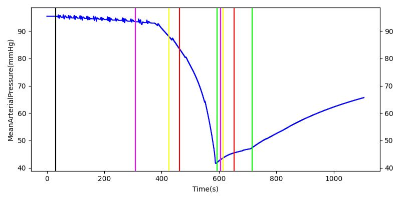
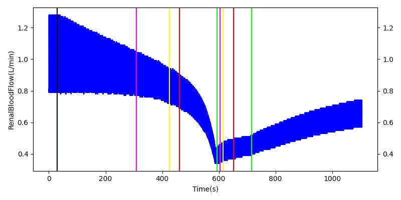
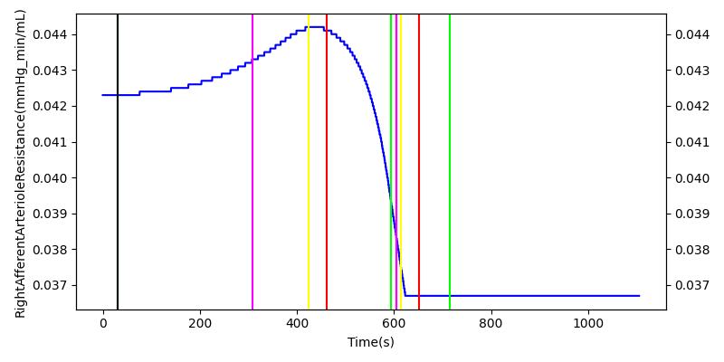
Hemorrhage - Action
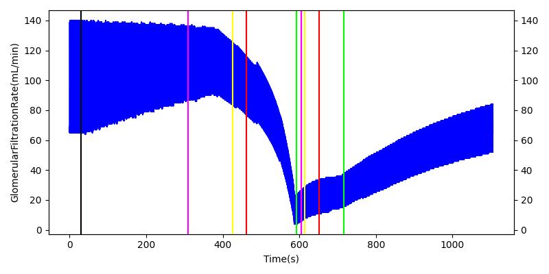
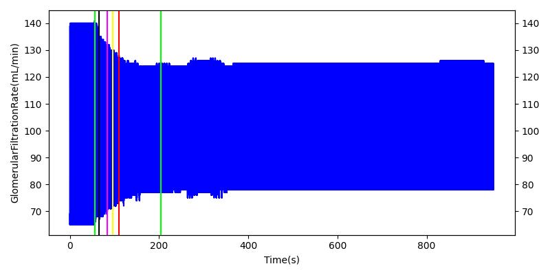
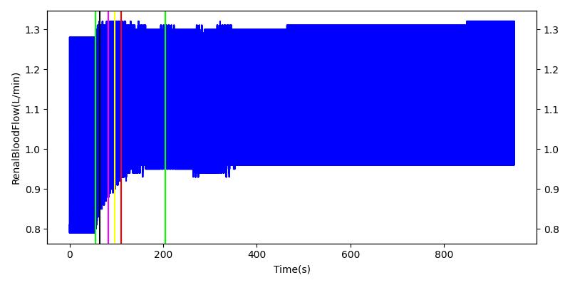
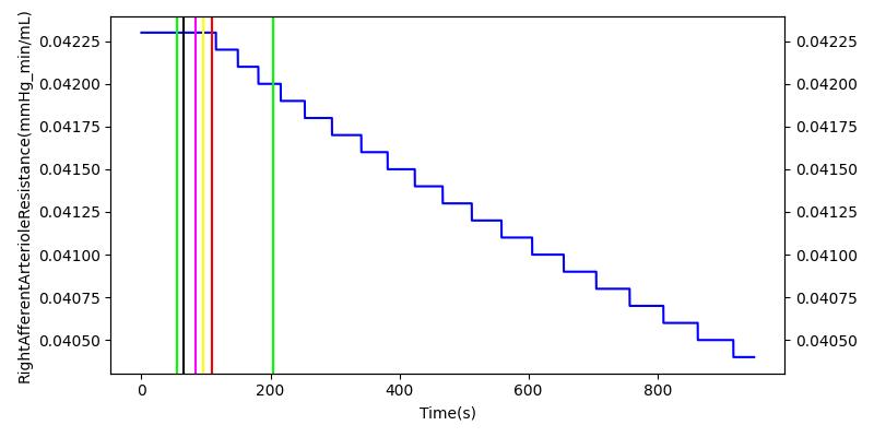
The renal system regulates glomerular filtration and renal blood flow through the tubuloglomerular feedback mechanism. This mechanism is modeled through constriction and dilation of the afferent arteriole as a function of sodium flow rate into the tubules. This mechanism is tested through two different hemorrhage scenarios. As the patient bleeds, blood volume and mean arterial pressure decrease, causing a reduction in blood flow to the renal system. As this decrease happens, the TGF system tries to compensate by dilating the afferent arteriole, reducing the resistance to flow into the glomerular capillaries. This balances the filtrate up to a point, but as blood volume and pressure continue to decrease, renal blood flow and glomerular filtration rate see reductions in line with past research [68]. This is more pronounced as the hemorrhage is allowed to persist. Qualitatively, the renal system in engine displays the mechanical trends seen in past research.
Table 9 shows the effect seen in the Renal system. For a complete write-up of the hemorrhage scenarios, see the Cardiovascular Methodology.
| Action | Notes | Action Occurrence Time (s) | Sampled Scenario Time (s) | Glomerular Filtration Rate (mL/min) | Mean Arterial Pressure (mmHg) | Renal Blood Flow(mL/min) | Urine Production Rate (mL/min) |
|---|---|---|---|---|---|---|---|
| Initiate 140 mL/min Hemorrhage | 30 | 600 | Decrease [68] | Decrease [68] | Decrease [68] | Decrease [68] | |
| Stop Hemorrhage | 620 | 1000 | Slight Increase [68] | Steady [68] | Slight Increase [68] | Steady [68] |
For the class III hemorrhage, the renal function displays the same trends but with a further reduction in glomerular filtration and renal blood flow due to the duration of the bleed action.
| Action | Notes | Action Occurrence Time (s) | Sampled Scenario Time (s) | Glomerular Filtration Rate (mL/min) | Mean Arterial Pressure (mmHg) | Renal Blood Flow(mL/min) | Urine Production Rate (mL/min) |
|---|---|---|---|---|---|---|---|
| Initiate 250 mL/min Hemorrhage | 30 | 600 | Decrease [68] | Decrease [68] | Decrease [68] | Decrease [68] | |
| Stop Hemorrhage | 605 | 1000 | Slight Increase [68] | Steady [68] | Slight Increase [68] | Steady [68] |
 |  |
 |  |
 | |
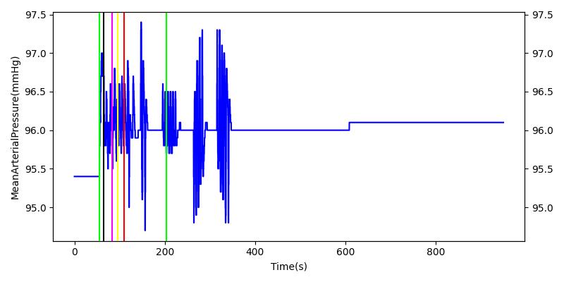
High Altitude - Action
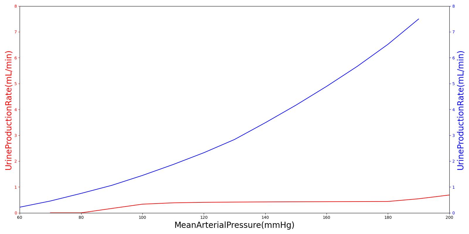
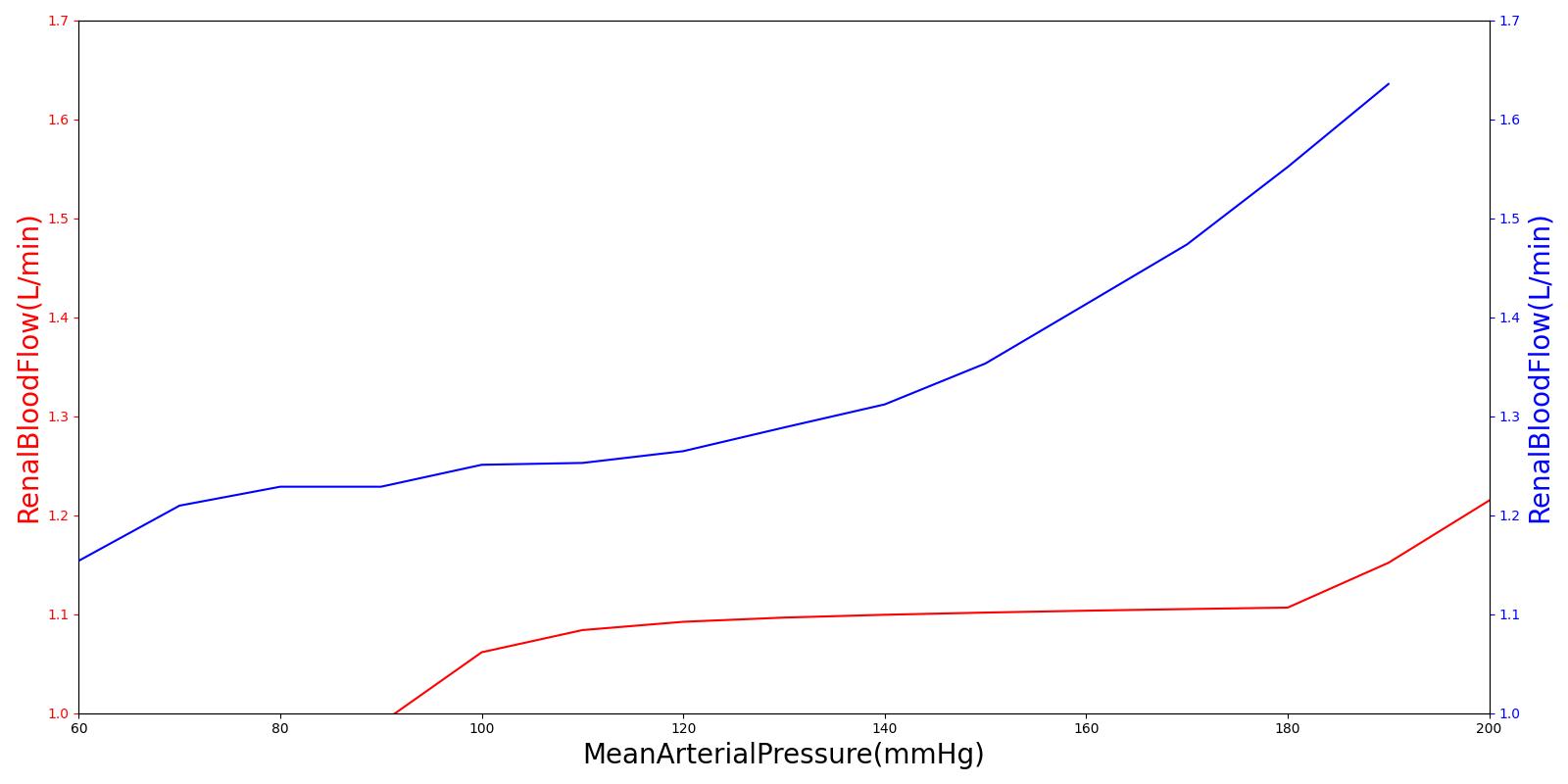
After a rapid change in altitude, epinephrine is released in response to the O2 deficit in the myocardium. This causes an increase in mean arterial pressure, which triggers a renal tubuloglomerular feedback response. The afferent arteriole resistance increases in an attempt to maintain GFR and renal blood flow. The MAP increases quickly and stabilizes at approximately 110 mmHg, which causes initial increases in GFR and Renal Blood Flow. These changes are quickly accounted for through the regulation from the tubuloglomerular feedback as expected.
Table 11 shows the effect seen in the Renal system. For a complete write-up of the High Altitude scenario see the Energy Methodology.
| Action | Notes | Action Occurrence Time (s) | Sampled Scenario Time (s) | Glomerular Filtration Rate (mL/min) | Renal Blood Flow(mL/min) | Urine Production Rate (mL/min) |
|---|---|---|---|---|---|---|
| Initiate Environment Change | 50 | 900 | Slight Increase [152] | Slight Increase [152] | Increase [152] |
 |  |
 |  |
 | |
Renal Stenosis - Condition
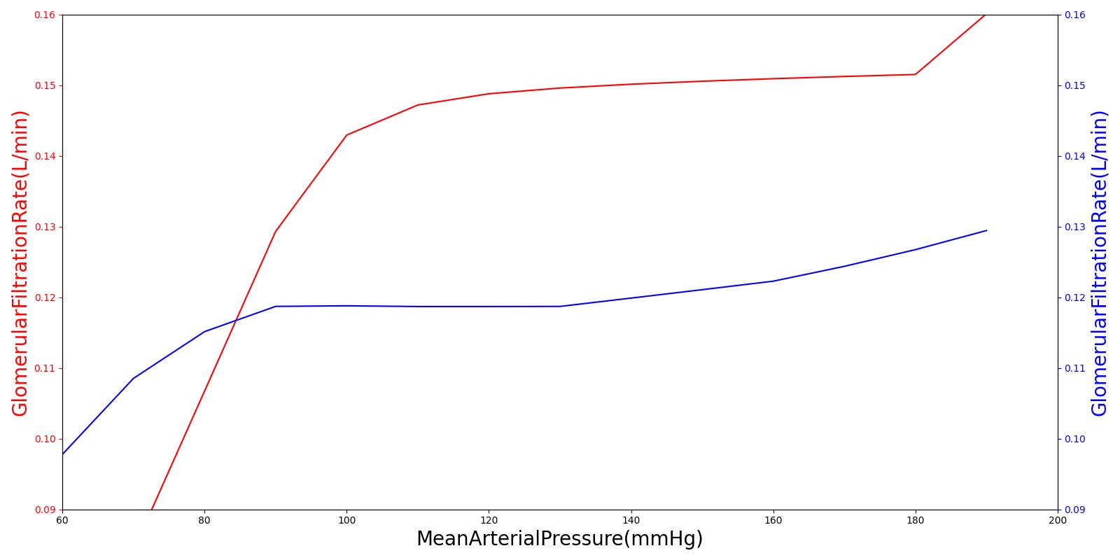
The Renal Stenosis condition is validated against two different scenarios, testing severity and location of the condition. The moderate unilateral stenosis places a 60 percent severity on the left kidney and none on the right. The direct effect of a stenosis is a seen through a decrease in renal blood flow and glomerular filtration rate. Total vascular resistance and mean arterial pressure is increased because of the increased resistance on the renal artery. This causes a drop in cardiac output via the baroreceptor feedback response to the increased vascular resistance. The blood volume is steady in the engine due to a lack of angiotensin 2 and aldesterone hormonal responses.
| Condition | Notes | Sampled Scenario Time (s) | Blood Volume (mL) | Systemic Vascular Resistance (mmHg/mL/s) | Cardiac Output (mL/min) | Mean Arterial Pressure (mmHg) | Systolic Pressure (mmHg) | Diastolic Pressure (mmHg) | Renal Blood Flow (mL/min) | GFR (mL/min) |
|---|---|---|---|---|---|---|---|---|---|---|
| Renal Stenosis | 60% unilateral occlusion of kidneys | 120 | Increase [199] | Increase [199] | Mild decrease [12] | Increase [75] | Increase [75] | Increase [75] | Decrease [361] | Decrease [361] |
The severe bilateral stenosis condition tests the effects of kidney function due to a 90 percent increase in renal artery resistance on both kidneys. Like the unilateral condition, the kidney and cardiovascular function meet validation. A more pronounced decrease in renal blood flow and glomerular filtration rate can be seen due to the increased severity of the stenosis.
| Condition | Notes | Sampled Scenario Time (s) | Blood Volume (mL) | Systemic Vascular Resistance (mmHg/mL/s) | Cardiac Output (mL/min) | Mean Arterial Pressure (mmHg) | Systolic Pressure (mmHg) | Diastolic Pressure (mmHg) | Renal Blood Flow (mL/min) | GFR (mL/min) |
|---|---|---|---|---|---|---|---|---|---|---|
| Renal Stenosis | 90% bilateral occlusion of kidneys | 120 | Increase [199] | Increase [199] | Mild decrease [12] | Increase [75] | Increase [75] | Increase [75] | Decrease [361] | Decrease [361] |
Conclusions
The engine has implemented a functional renal model in conjunction with a whole-body physiology engine. Even with the simplified single-node nephron model, the system is able to accurately follow the overall renal transport of fluid and substances. The capabilities of the renal model allow for fluctuations in urine production rate, changes in blood pressure, and variations in clearance rates, as well as allowing for autogregulation with accurate responses to pressure changes and sodium concentration changes in the tubules.
Future Work
Coming Soon
These additions are expected in the near future:
- Acid-base balance reinvestigation
- Improvements to make the Cardiovascular and Renal systems more independent and modular
- Better handeling of substance clearance
Recommended Improvements
These are some recommended improvements and additions:
- Peristalsis model
- Insulin as an optional substance for kidney validation/verification
- Remaining urinalysis substances
- Renin and angiotensin control
- Handle drugs similarly to metabolites
- Model kidney failure
- Catheterization
- Kidney stones
- Dialysis machine model
- Add dehydration and starvation for further Renal System validation
Appendices
Glossary
BUN - Blood Urea Nitrogen
GFR - Glomerular Filtration Rate
IV - Intravenous
MAP - Mean Arterial Pressure
RBC - Red Blood Cells
WBC - White Blood Cells
mL - Milliliters
min - Minutes
kg - Kilograms
g - Grams
ug - Micrograms
L - Liters
mol - Moles
mOsm - Milliosmoles
mmHg - Millimeters of Mercury
Data Model Implementation
Compartments
- LeftKidney
- LeftRenalArtery
- LeftNephron
- LeftAfferentArteriole
- LeftEfferentArteriole
- LeftGlomerularCapillaries
- LeftBowmansCapsules
- LeftTubules
- LeftRenalVein
- RightKidney
- RightRenalArtery
- RightNephron
- RightAfferentArteriole
- RightEfferentArteriole
- RightGlomerularCapillaries
- RightBowmansCapsules
- RightTubules
- RightRenalVein
- Ureters
- LeftUreter
- RightUreter
- Bladder