Overview

Abstract

The cardiovascular system is a closed-loop system of compartments that represents the human circulatory system. The cardiovascular system is sometimes described as two separate circulations: the systemic circulation and the pulmonary circulation. Both circulations are represented in the Cardiovascular system, as well as the lymph. The dynamical state of the Cardiovascular System is determined at every timestep through a three-step process. First, intra- and inter-system feedback is applied during the preprocess step. Next, the state of the circulatory system is determined by solving an equivalent circuit. Finally, the state of the system is updated in preparation of time advancement. Through system and action validation, we demonstrate the accuracy of the model at resting physiology and a variety of cardiovascular related insults and interventions with appropriate system feedback.

Introduction

Cardiovascular Physiology

The cardiovascular system is a large organ system comprised of the heart and the blood vessels. It serves as the body's primary transport and distribution system. The cardiovascular system is sometimes described as two separate circulations: the systemic circulation and the pulmonary circulation. In the systemic circulation, oxygenated blood leaves the left side of the heart, travels through arteries and into the capillaries, and then returns as deoxygenated blood through the veins to the right side of the heart. From the right side of the heart, the deoxygenated blood travels in the pulmonary circulation through the pulmonary arteries, is re-oxygenated in the pulmonary capillaries, and then returns to the left side of the heart through the pulmonary veins (Figure 1). Whether the cardiovascular circulation is thought of as one closed circuit with a single dual-purpose pump or two interconnected circuits with separate synchronous pumps, the key combination of systemic and pulmonary vasculature serves as a distribution and exchange network, providing vital oxygen to the tissues and removing toxic carbon dioxide while distributing nutrients and other substances necessary for healthy physiologic function.

Figure 1. The cardiovascular System with pulmonary and systemic circulations of the human body [371]. Both the pulmonary and systemic circulation originate in the heart, which acts as a pump driving the blood through the entire body. The blood then returns to the right heart via the vena cava, where the right ventricle sends it to the pulmonary arteries and into the lungs. Gas exchange occurs in the vascular arterioles, creating oxygen-rich blood. This blood then returns via the pulmonary veins to the left atrium of the heart. The oxygen-rich blood enters the systemic circulation, providing oxygen to the rest of the body.

The cardiovascular system is one of two systems that comprise the circulatory system, the other being the lymphatic system. The cardiovascular system includes a low-resolution lymphatic circulation. Because the resolution of the lymph circulation in the engine is considerably lower than the resolution of the cardiovascular circulation, we refer to the comprehensive circuit as the circulatory circuit, but we maintain the term cardiovascular as system nomenclature to highlight the modeling focus. In other words, the lymph circulation is not a physiological model of the human lymphatic system. It only serves as an accessory return for interstitial fluid. More information about the lymph model and the other accessory advection models is available in the Tissue Methodology report.

Cardiovascular Modeling

Brief Introduction to Cardiovascular Modeling

Cardiovascular (CV) models range from high-resolution, small-region-of-interest models [359] [390] [122] to low-resolution, whole-body simulations [166]. Increased resolution may provide a more accurate solution in a localized region at the expense of decreasing the modeling region. However, the level of accuracy achieved with this model is not always required to answer the question posed. Three-dimensional (3D) computational fluid dynamics (CFD) models are generally limited to short segments of the arterial or venous tree due to high computational requirements. These high-resolution models are well-suited for investigating complex geometries following surgical intervention, such as the Fontan Circulation [397] [77]. However, they are not suitable for modeling long-term or systemic effects in the CV System [362] because it is only feasible to simulate a few cardiac cycles.

One-dimensional (1D) models can also predict the pressure and flow wave dynamics within a region of interest [405] [406] and have the advantage of a lower computational cost than full CFD models. Like CFD models, 1D models begin with the Navier-Stokes equations, but they are reduced to a hyperbolic partial differential equation by including an axisymmetric assumption. The resultant equation dictates a constant pressure in the radial direction if the radius of the vessel is small relative to a characteristic wave length [51]. These models are well-suited for investigating specific CV problems [345] [64] and have been coupled with dynamic downstream effects to investigate problems over numerous cardiac cycles [65]. However, the computational cost associated with 1D models still renders them unsuitable for modeling the complete closed-circuit dynamics of the circulation over the entire range of vessel diameter and lengths in the human body.

The lumped parameter method of hemodynamic modeling assumes characteristics of organ vessels or vessel segments can be “lumped” into representative parameters. For instance, the viscosity of a fluid can be lumped together with the geometry of a vessel segment to derive an effective resistance to blood flow. If a tube is rigid, the pressure-flow dynamics are completely characterized by the resistance to flow in the tube. If a tube is elastic, an additional compliance parameter is used to characterize the impedance and calculate the pressure-flow dynamics in the segment. In humans, small arteries can be approximately rigid [272], and the corresponding veins can be significantly more compliant (24 times more compliant) [156].

Otto Frank first formulated the quantitative model (called a Windkessel model after the wave-filtering air chamber in archaic firefighting equipment) relating systemic blood pressure with vessel elasticity [123]. In the analogous electrical circuit (see Circuit Methodology), the Windkessel model includes a capacitor, representing the compliance of the artery, connected in parallel with a resistor, representing the resistance to flow through the vessel. An alternate three-element form of the Windkessel model was developed by Westerhof et al. [394] that included a black-box, two-terminal input circuit, represented as an additional resistor, to quantify the characteristic impedance of the arterial tree. Similar applications of the electric analogue circuit have been applied to form CV circuits that can be classified as multi-segment or multi-system models.

Lumped Parameter Model

Lumped parameter models have proven suitable for larger-scale, longer time-scale simulations due to lower computational requirements and sufficient fidelity. A multi-organ model can run in real time while still producing an accurate blood pressure and flow waveform prediction. The drawback to this type of model is the large number of parameters requiring definition or tuning. However, significant work has been targeted at determining appropriate parameter values [42] [202] [246] [272] [305] [395]. This body of work, in particular Heldt’s open source CV simulator that includes lumped parameter models [166] [169] [355], supports the decision to implement these models in the engine.

System Design

Background and Scope

History of the Cardiovascular Model

The CV Model has its origins in Guyton's four-compartment (three vascular, plus one heart) model of the CV System designed to analyze the effect of varying circulatory factors on cardiac output [153]. Rideout, et al. used Guyton’s foundation and an electric-hydraulic analogy to streamline the generation of difference-differential equations for modeling fluid flow in distensible vessels [305]. Yasuhiro Fukui leveraged the previous work to model the CV and respiratory systems and their interactions [126]. The development of a mass and momentum transport model of the CV System allowed for the simulation of interactions between the CV System and angiotensin [237]. Following the success of the angiotensin-cardiovascular simulator, development of the drug-interaction model continued and eventually led to an anesthesiology simulator that incorporated CV, respiratory, and drug models [342]. This simulator, released by Advanced Simulation Corporation as Body Simulation for Anesthesia™, formed the backbone of the HumanSim™ physiology engine, which continues to provide realistic physiology for several serious training games in the HumanSim product line, including HumanSim: Sedation and Airway [293]. The HumanSim physiology engine is the starting-point for the engine. The basic building blocks of the CV System remain as described in Masuzawa et al. [237]; however, the CV circuit has been further developed to provide a more accurate CV simulation and drive other systems through intersystem dependencies.

Data Flow

The state of the CV System is determined at every time step through a three-step process: Preprocess, Process, and Postprocess. In the Preprocess step, feedback from other systems, as well as intrasystem feedback, is processed in preparation for determining the state of the system. Process uses the circuit calculator to compute the new state of the system. Postprocess is used to prepare the system for the advancement of time. More specifics about these steps are detailed below.

Initialization and Stabilization

First, the patient-specific homeostatic state of the cardiovascular circuit is computed. Next, all system parameters are initialized. The Cardiovascular System is then initialized to the resting state. Conditions are then applied by modifying system and patient parameters and restabilizing the engine. The available conditions in the Cardiovascular System are anemia, heart failure, pericardial effusion, and pulmonary shunt.

Tune Circuit

In the tune circuit step, the resistors and capacitors associated with tissue compartments are tuned during stabilization to achieve the mean arterial pressure given in the patient file.

Preprocess

Begin Cardiac Cycle

Cardiac cycle calculations include methodology for updating the driving force (heart contraction and relaxation) of the CV System throughout the duration of a CV cycle (a single heart beat). This includes a set of systolic calculations that updates contractility at the beginning of the cycle to represent a heart contraction. Modifications to heart rate and heart compliance are calculated by BeginCardiacCycle and applied for the remainder of the current cardiac cycle. Changes to things like heart rate and heart contractility can only occur at the top of the current cardiac cycle after the last cardiac cycle has completed. This helps to avoid discontinuous behavior such as the complete cessation of heart function mid-contraction.

Calculate Heart Elastance

This method tracks the progress of the current cardiac cycle and modifies the compliance of the left and right heart to drive the cardiovascular circuit. The reduced compliance at the beginning of the cycle acts to increase the pressure, driving flow out of the heart. The compliance is then reduced, allowing flow into the heart. The reduction and increase in compliance represents the systolic and diastolic portions of the cardiac cycle, respectively. The compliance is driven by a Hill-type elastance equation [104].

Process Actions

Process Actions modifies the CV parameters and circuit properties due to actions (insults or interventions) specified by the user. The actions found in the action process are: CPR, hemorrhage, pericardial effusion, and cardiac arrest.

Process

The generic circuit methodology developed for the engine is used to solve for the pressure, flow, and volume at each node or path in the equivalent circuit. For more details, see Circuit Methodology.

Calculate Vital Signs

This function takes the current timestep’s circuit quantities to calculate important system-level quantities for the current time step. The system pressures and flow rates related to shunting are calculated here. In addition, the events hypovolemia, tachycardia, bradycardia, and asystole are triggered in this function.

Postprocess

The Postprocess step moves everything calculated in Process from the next time step calculation to the current time step calculation. This allows all other systems access to the information when completing their Preprocess analysis for the next time step.

Assessments

Assessments are data collected and packaged to resemble a report or analysis that might be ordered by a physician. No assessments are associated with the Cardiovascular system.

Features, Capabilities, and Dependencies

The Cardiovascular Circuit

The CV circuit (Figure 2) estimates blood pressure, flow, and volume for organs that are represented by several compartments. These compartments are comprised of lumped parameter models that use resistors and capacitors. Inductors may also be used to model inertial effects. The system is discretized into nodes that are connected by paths (see Circuit Methodology). The circuit used to represent the CV System was designed to provide a level of resolution and fidelity that meets the requirements of the overall project.

For example, to provide a means for clearing drugs and substances from the bloodstream, the liver and kidneys must have blood flow, pressure, and volume calculations. Another example is the four extremities (right and left arms and legs) that provide extremity hemorrhage capabilities, having been implemented in a previous project (HumanSim: Combat Medic). In this way, the lumped parameter model provides a mechanism for increasing fidelity as required by the anatomic region or physiologic condition being modeled. The large thoracic arteries are lumped together into one “Aorta” compartment, which is represented by four nodes and three paths. The fidelity of any compartment could be easily improved by increasing the level of discretization. By adding nodes and paths, the engine “Aorta” could become the “Ascending Aorta” and “Descending Aorta” to accommodate the fidelity demands of the other systems. This could provide an opportunity to model more complex geometries and pathologies, such as stenosis. Figure 2 shows the cardiovascular circuit. For clarity, the more discretized renal circuit is not shown in this diagram.

Figure 2. The cardiovascular circuit consists of nodes that are connected via paths. These segments of nodes and paths are mapped to several compartments which represent the anatomy of the cardiovascular system. The circuit is used to estimate the blood pressure, flow, and volume of these anatomical compartments.

Nodes serve as the connection points for paths and are the locations at which pressures are measured. Each CV node contains a pressure value, which is given with respect to the atmospheric reference node (indicated in the diagram by the equipotential symbol). Paths contain information about the flow (volume per time). The Circuit Methodology document contains more information about circuit definitions and modeling. The Substance Transport Methodology contains more information about the substance transport. In general, nodes contain "across" information and paths contain "through" information.

The elements of the CV circuit are used to model the fluid dynamics of the human CV System (hemodynamics). The hemodynamic pressure and flow are calculated from the lumped parameters that are determined by the circuit element. The equations used to calculate pressure and flow are shown below. These equations are automatically generated and solved simultaneously by the Circuit Solver.

Derived values for the hemodynamic parameters are available, particularly for specific vessel segments [272] [306]. However, in the engine, these parameters are tuned to provide the physiologic response of a given patient profile. We completed the tuning process by choosing estimates for each parameter value based on the existing system values (Body and HumanSim) or based on physiologic data. We then analyzed the model outputs and adjusted parameters to obtain organ and system-level outputs that satisfied the validation requirements. The Results and Conclusions section describes validation in more detail.

The Heart

The heart model generates pressure that drives the hemodynamics through a variable capacitor that simulates the changing elastance of the myocardium throughout the cardiac cycle. The simulated heart has two sides, left and right, simulating the two sides of the human heart. The atria are not included in the heart model; only the ventricular behavior is modeled.

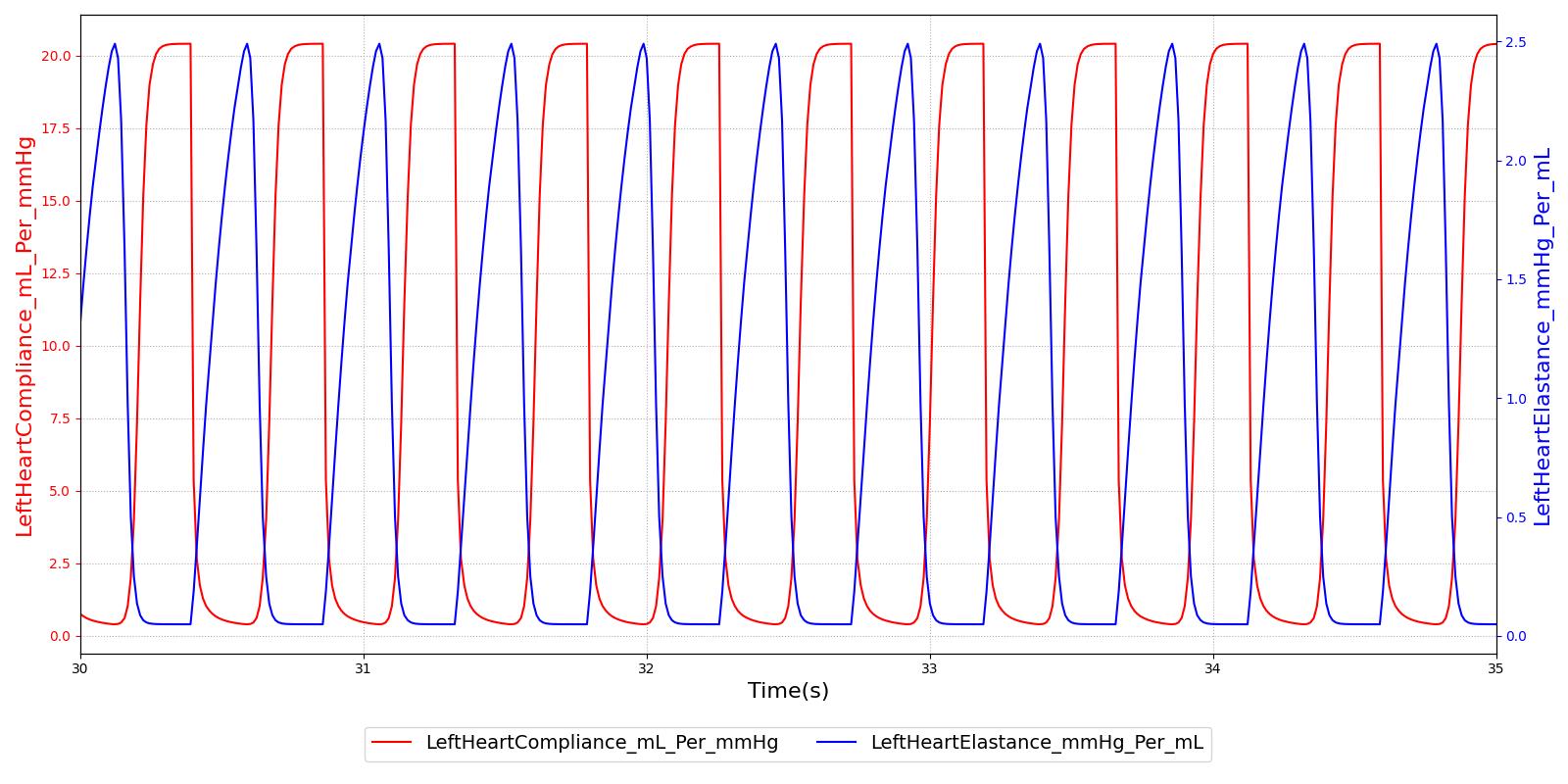
Heart Elastance and Compliance

The heart compliance is calculated from the inverse of the heart elastance. The heart elastance model used is adapted from the one developed by Stergiopulos et al [104]. This model utilizes a double Hill function to represent heart elastance over the cardiac cycle time period. It was chosen due to its ability to scale with increasing or decreasing cardiac cycle times. The functional form for elastance of both left and right ventricles is shown in Equation 1 and Equation 2.

$E_{v} (t)=(E_{\max ,v} -E_{\min ,v} )\left(\frac{f(t)}{f_{\max } } \right)+E_{\min ,v}$

Equation 1.

Where *E_max,v* is the maximum ventricle elastance in mmHg per mL. *E_min,v* is the minimum ventricle elastance in mmHg per mL. f(t) is the double Hill function, and *f_max* is the maximum value of the double Hill over the cardiac cycle length.

$f(t)=\left[\frac{\left(\frac{t}{\alpha _{1} T} \right)^{n_{1} } }{1+\left(\frac{t}{\alpha _{1} T} \right)^{n_{1} } } \right]\left[\frac{1}{1+\left(\frac{t}{\alpha _{2} T} \right)^{n_{2} } } \right]$

Equation 2.

Where α₁ , α₂ , *n₁*, and *n₂* are shape parameters used to determine the distribution of the double Hill function. T is the cardiac cycle time period and t is the current time within the cardiac cycle.

The relationship between the elastance and compliance in the engine is shown in Figure 3.

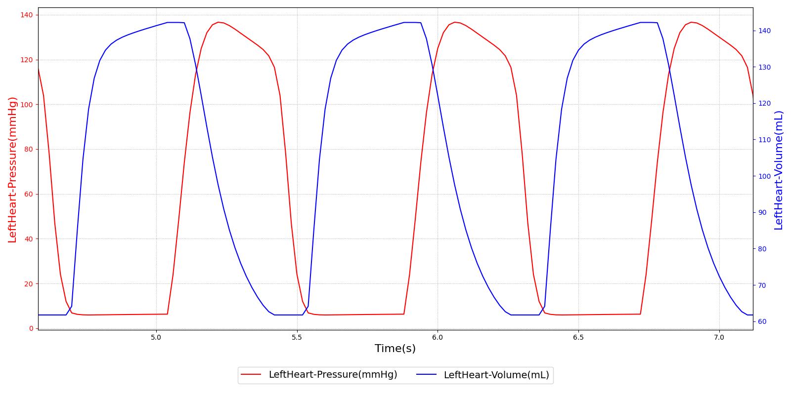
Figure 3. The left heart compliance and elastance are shown to be inversely related to each other. The elastance represents the change in pressure per change in volume, while the compliance is the change in volume per change in pressure. These quantities define the contraction of the heart, which drives the pressure and flow of the cardiovascular circuit.

Heart Pressure, Volume, and Flow

The variable compliance, which is used to model heart contraction and relaxation, yields pressure and volume changes that drive the flow through the CV circuit. This variable compliance driver allows the pressures and volumes to be calculated within the heart, as shown in Figure 4.

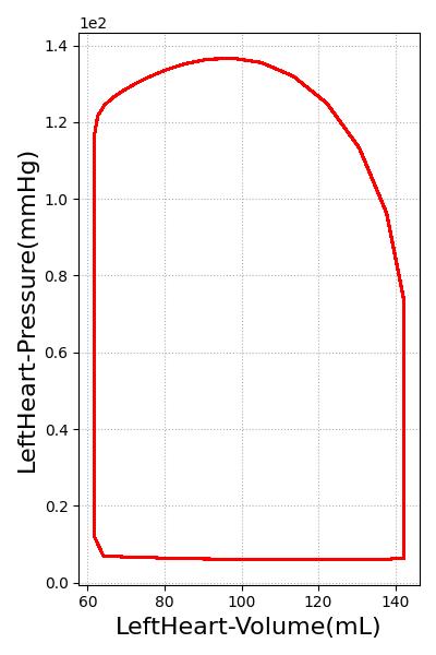
Figure 4. Relationship between pressure and volume in the left heart throughout the cardiac cycle. The relaxation of the heart muscle is modeled by increasing the compliance, resulting in an increase in left heart volume with a relatively constant left heart pressure. The contraction is represented by a rapid decrease in the compliance, leading to large pressure increases for small volume additions. This large pressure value drives the fluid out of the heart with flow rates calculated based on the circuit solution.

A pressure-volume curve is used to represent the evolution of the cardiac cycle from the systolic contraction to diastolic relaxation. The pressure-volume curve for the left ventricle is shown in Figure 5. Starting from the bottom left and moving clockwise, the curve demonstrates a rapid increase in pressure with no change in volume. This indicates the systolic contraction of the cardiac cycle. Following this, the pressure declines rapidly as the heart expands during diastole. The last portion of the curve shows decreasing volume at constant pressure. Normally, the pressure would decrease slightly due to the imperfect mitral valve, which does not close instantly. The engine uses ideal valves, which close instantaneously, causing the pressure to be maintained as volume decreases.

Figure 5. The pressure-volume curve for the left ventricle is represented as a pressure vs. volume plot. It demonstrates the the contracting and relaxing portions of the cardiac cycle. In addition, the curve demonstrates the use of ideal valves in the simulated heart due to instantaneous changes in volume at a set pressure.

Drug Effects

As drugs circulate through the system, they affect the Cardiovascular System. The drug effects on heart rate, mean arterial pressure, and pulse pressure are calculated in the Drugs System. These effects are applied to the heart driver by incrementing the frequency of the heart based on the system parameter calculated in the Drugs System. Additionally, the mean arterial pressure is modified by incrementing the resistance of the blood vessels. At each timestep, the resistors are incremented on each cardiovascular path. In the future, the pulse pressure will be modified by changing the heart elastance. However, no drugs had pulse pressure changes; therefore, this step has not been necessary. The strength of these effects are calculated based on the plasma concentration and the drug parameters in the substance files. For more information on this calculation, see Drugs Methodology.

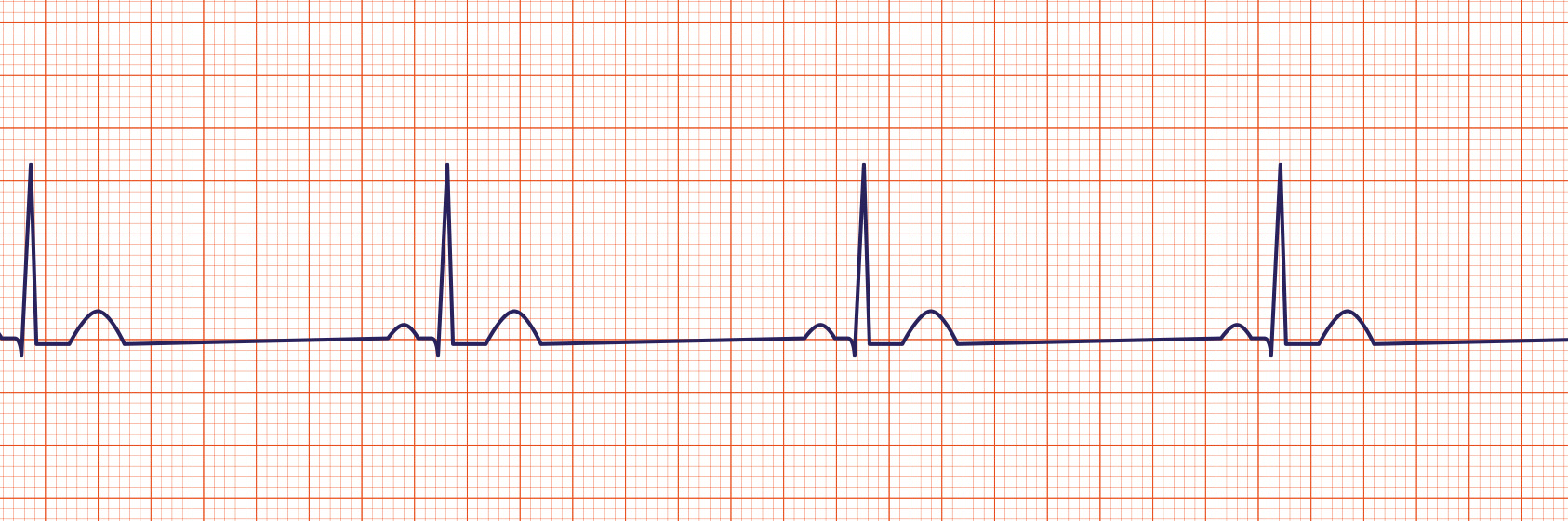
Electrocardiogram

The engine electrocardiogram (ECG) machine outputs an ECG waveform to represent the currently supported heart rhythms. The waveform is not a calculated value; the current ECG system does not model the electrical activity of the heart. This data is stored in a text file. To account for the variable heart rate, rhythms are time series of voltage that is representative of a single cardiac cycle. The points are then interpolated based on the length of the cardiac cycle.

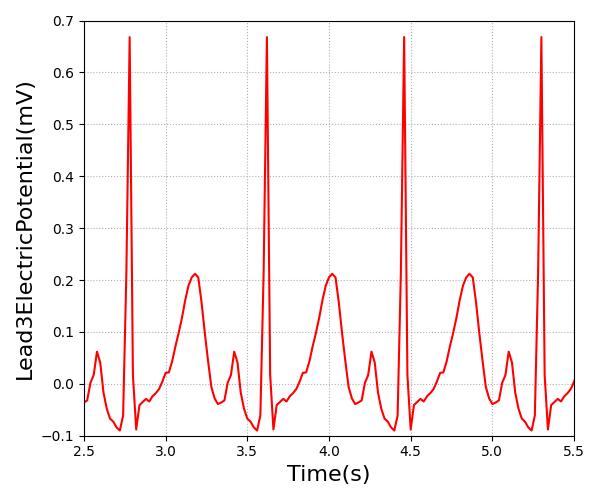
Figure 6 shows the lead 3 sinus waveform in Pulse compared to an example sinus waveform with the key features highlighted.

Figure 6. The ECG system produces a normal sinus waveform with the expected features.

Patient Variability

The cardiovascular system is heavily dependent on the patient. The cardiovascular circuit parameters are all set based on the patient configuration. For example, the proportion of blood flow to the fat compartment depends on the sex of the patient, and the initial flow proportions dictate initial vascular resistance. Likewise, the volume of the fat compartment depends on the sex, body fat fraction, height, and weight of the patient, and the initial volume and pressure are used to compute the initial vascular compliance for paths associated with a compartment. After initial values are computed, the cardiovascular circuit parameters are adjusted to meet target pressures, which are also specified in the patient file. Because the cardiovascular system is profoundly dependent on the patient configuration, several stabilization iterations are sometimes necessary to achieve a specific desired state. For that reason, we make modifications to the parameters to move the circuit closer to a Standard patient state to speed stabilization for that patient, and other custom states may require longer stabilization periods. A detailed discussion of patient configuration and variability is available in the Patient Methodology report.

Dependencies

The other engine systems depend on the CV System to function accurately and appropriately. The CV System provides the medium (blood) and the energy (pressure differentials and subsequent flow) to transport substances throughout the engine. A complete list of substances and their descriptions can be found in the Substance Transport Methodology. Similarly, the CV System is dependent on all of the other systems. Feedback from other systems influences the cardiac behavior via heart rate and elastance modifiers and the systemic circulation through resistance modifications to the circuits. For example, as the plasma concentration of a drug increases, the elastance of the heart, heart rate, and systemic resistance are modified through the pharmacodynamic effects (multipliers), resulting in changes to the blood flow, pressure, and volume calculations. Additionally, baroreceptor feedback leads to modification of heart rate, elastance, and vascular resistance and compliance in order to regulate the arterial pressure. For more information on baroreceptor feedback see Nervous Methodology.

Gas exchange is one area that closely ties the respiratory system, substances, and the CV system together. Gas exchange is calculated based on the partial pressures of the gases in the lungs and the capillary beds (Substance Transport Methodology). If respiration was to stop due to a drug effect or physiologic condition, such as airway obstruction, the gas exchange calculations would be affected. Oxygen would stop diffusing into the CV System from the Respiratory System, resulting in an oxygen deficit in the cardiac tissue.

Assumptions and Limitations

The constant-compliance equations in the CV System assume a linear diastolic pressure-volume relationship in the vessels (ΔV = CΔP) representative of an elastic vessel wall. This assumption is appropriate for many blood vessels under normal physiologic conditions; however, research shows that many vessel walls are more appropriately modeled as visco-elastic walls [11]. While the non-linear pressure-volume relationship within the heart is modeled using a variable capacitor, the visco-elastic nature of the blood vessels is not addressed in this model. Rigid and elastic wall properties have been used to model the hemodynamic behavior in high-fidelity models with success [11]. Therefore, the level of fidelity of the lumped parameter model and resulting simulation support the use of elastic walls.

The CV model has a waveform limitation because of our ideal diode model. We assume the valves are perfect Booleans. In reality, there is a transition time between the open and closed states of a valve. During this time, a small amount of retrograde flow may be present [292] . In the future, we hope to incorporate retrograde flow through a Zener diode. However, the current methodology does allow retrograde flow at any location without a diode. The Zener diode implementation will provide a mechanism for future modeling efforts, including abnormal heart valves that result in significant retrograde flow.

Conditions

Anemia

Anemia conditions reduce the oxygen-carrying capacity of the blood. The engine models iron deficiency anemia as a chronic condition, which is characterized by a decrease in hemoglobin concentration and subsequent decreases in hematocrit and blood viscosity [92]. These factors lead to a decrease in systemic vascular resistance [152]. The engine currently supports up to a 30% decrease in hemoglobin. After engine stabilization, the chronic condition reduces the hemoglobin throughout the circuit and reduces the systemic vascular resistance to represent the change in viscosity. The engine then re-stabilizes based on the chronic condition criteria. For more information, see System Methodology. There is an observable increase in venous return due to the decreased systemic vascular resistance. As validation data supports, there are no observable effects from the decreased oxygen-carrying capacity at rest. These effects will be evident in the future with incorporation of exercise. This condition is currently not validated.

Heart Failure

Heart failure refers to a malfunctioning of the heart, resulting in inadequate cardiac output. The current mode of heart failure being modeled in the engine is chronic left ventricular systolic dysfunction. After engine stabilization, the chronic heart failure is modeled with a 45% reduction in the contractility of the left heart. After the engine has re-stabilized using the chronic condition criteria (System Methodology), the heart ejection fraction of 60% is reduced to 31% as noted in the validation data [57]. The reduced contractility leads to a decrease in heart stroke volume, which causes an immediate drop in the cardiac output and arterial pressures. The baroreceptor reflex responds with an increase in heart rate in an attempt to return mean arterial pressure to its normal value. This model is currently not validated.

Pericardial Effusion

A chronic pericardial effusion is an accumulation of fluid in the pericardial sac that surrounds the heart. This accumulation occurs over a long period of time, resulting in the body making some accommodation to these changes. The result is an increased pressure on the heart, which leads to strained performance. This performance strain is less severe than in an acute effusion. Due to this increasing pressure, there is a decrease in stroke volume, which leads to a decrease in cardiac output and arterial pressures. To compensate for reduced stroke volume, the baroreceptor response raises the heart rate in an attempt to restore cardiac output.

Pulmonary Shunt

The pulmonary shunt generally models an unspecified change in the amount of blood that is shunted away from alveolar gas exchange in the pulmonary capillaries. This will impair the gas diffusion that occurs between the cardiovascular and respiratory systems. The pulmonary shunt can be specified on either the right, left, or both pulmonary vasculature and specified with a severity between 0 and 1.

Actions

Insults

Arrhythmia

An arrhythmia is a deviation from normal cardiac heart rate and function.

Currently, we support ECG data for the following arrhythmias

Asystole
Sinus Tachycardia
Sinus Bradycardia
Pulseless Electrical Activity (PEA)
Coarse and Fine Ventricular Fibrillation
Stable and Unstable Ventricular Tachycardia
Pulseless Ventricular Tachycardia

We have an arrhythmia action with the type of arrhythmia as the input. All of the arrhythmias were implemented as types that can be specified as part of the arrhythmia action. In general, it takes about 60s to trasition between arrhythmia's.

Asystole

The transition to asystole is instantaneous. We set the heart rate to 0 to reflect a lack of cardiac function [2]. All feedback and imapcts from additional actions will NOT impact the hemodynamics of the cardiovascular system, as there is no hemodynamic activity during this arrhythmia.

Figure 7. The ECG waveform is set to 0 volts to represent the lack of electrical activity [2] in asystole.

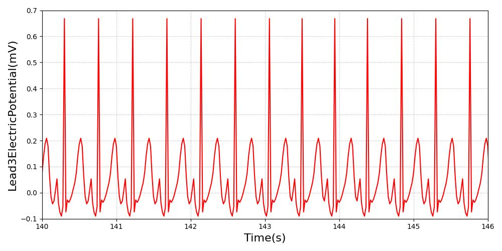
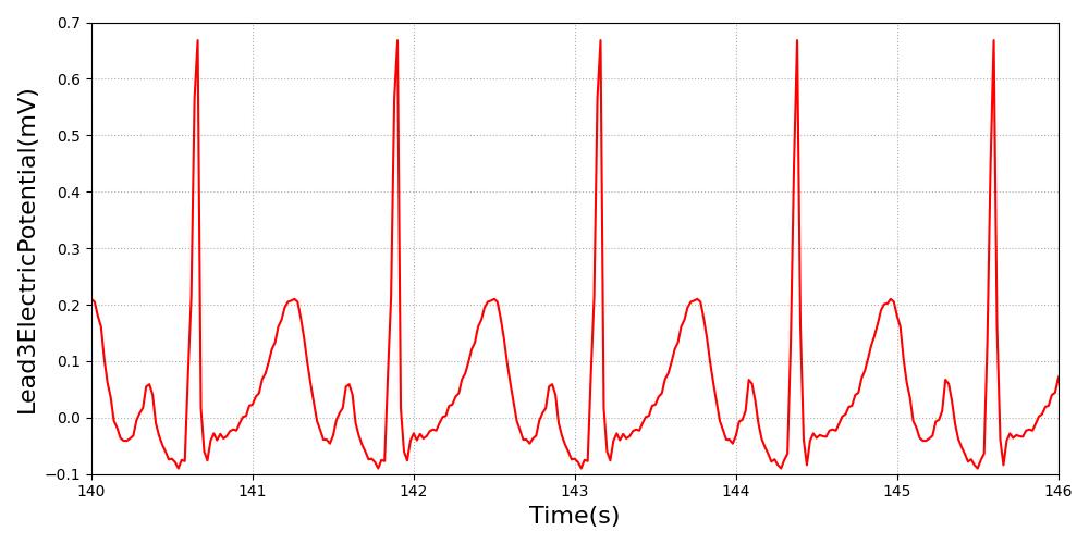
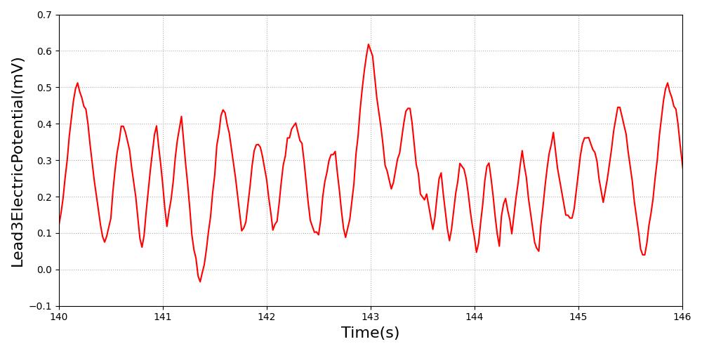
Sinus Tachycardia

The heart rate baseline is set to 130. Pulse will transition the patient to this heart rate over 60s. The ECG will use the shape of the normal sinus rhythm as its basis. As the heart rate baseline is modified, the output will update at the new heart rate frequency. All feedback and imapcts from additional actions will still impact the hemodynamics of the cardiovascular system from this new starting rate.

Figure 8. Due to the high heart rate, the engine output is summing together the P and T waves. In the image from PhysioNet, the output is not summed together as dramatically, due to the slight physiological compression of the waveform that the current ECG system and heart model do not support. [164] [137]

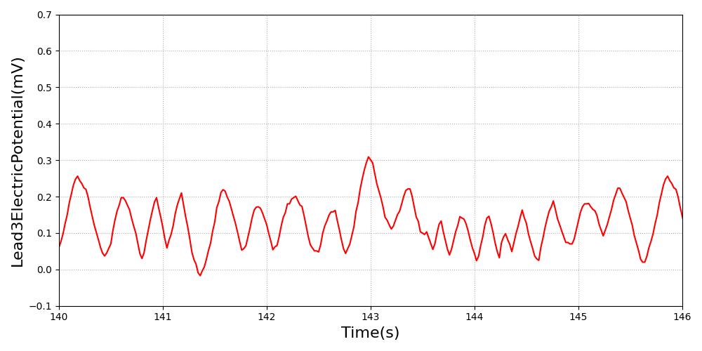
Sinus Bradycardia

The heart rate baseline is set to 50. Pulse will transition the patient to this heart rate over 60s. The ECG will use the shape of the normal sinus rhythm as its basis. As the heart rate baseline is modified, the output will update at the new heart rate frequency. All feedback and imapcts from additional actions will still impact the hemodynamics of the cardiovascular system from this new starting rate.

Figure 9. The increased R-R interval is evident in both waveforms. This is the primary indication of the low heart rate. Validation image courtesy of [385] .

Pulseless Electrical Activity (PEA)

Sinus pulseless electrical activity (PEA) is characterized by organized electrical activity of the heart, but no mechanical function [5]. For sinus PEA, the ECG is set to a normal sinus rhythm with a heart rate of 65 bpm; however, the amplitude of the waveform is reduced to reflect the weaker electrical activity [5]. The transition to PEA is instantaneous. All feedback and imapcts from additional actions will NOT impact the hemodynamics of the cardiovascular system, as there is no hemodynamic activity during this arrhythmia.

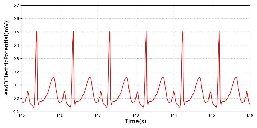
Figure 10. PEA is characterized by organized electrical activity in a normal sinus rhythm shape with a reduced amplitude [5].

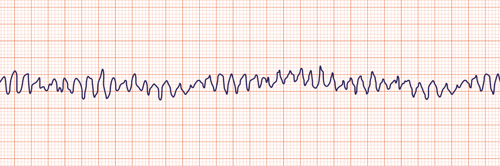
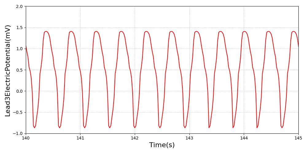
Ventricular Fibrillation Arrhythmias

Ventricular fibrillation is characterized by a lack of mechanical function of the heart and disorganized electrical activity [5]. As no cardiac cycle is associated with ventricular fibrillation, the ECG uses a representative period of disorganization (several seconds) was extracted from an arrhythmia database [286]. This representative dataset is then repeated throughout the duration of this arrhythmia. The transition to ventricular fibrillation is instantaneous.

Ventricular fibrillation is defined as either coarse or fine. Coarse ventricular fibrillation is represented by more electrical activity than fine ventricular fibrillation. The amplitude is reduced to half for fine ventricular fibrillation rhythm. All feedback and imapcts from additional actions will NOT impact the hemodynamics of the cardiovascular system, as there is no hemodynamic activity during this arrhythmia.

Figure 11. Ventricular fibrillation is characterized by disorganized electrical activity. Coarse (Left) has higher electrical signal than fine (Right) ventricular fibrillation [63].

Ventricular Tachycardia Arrhythmias

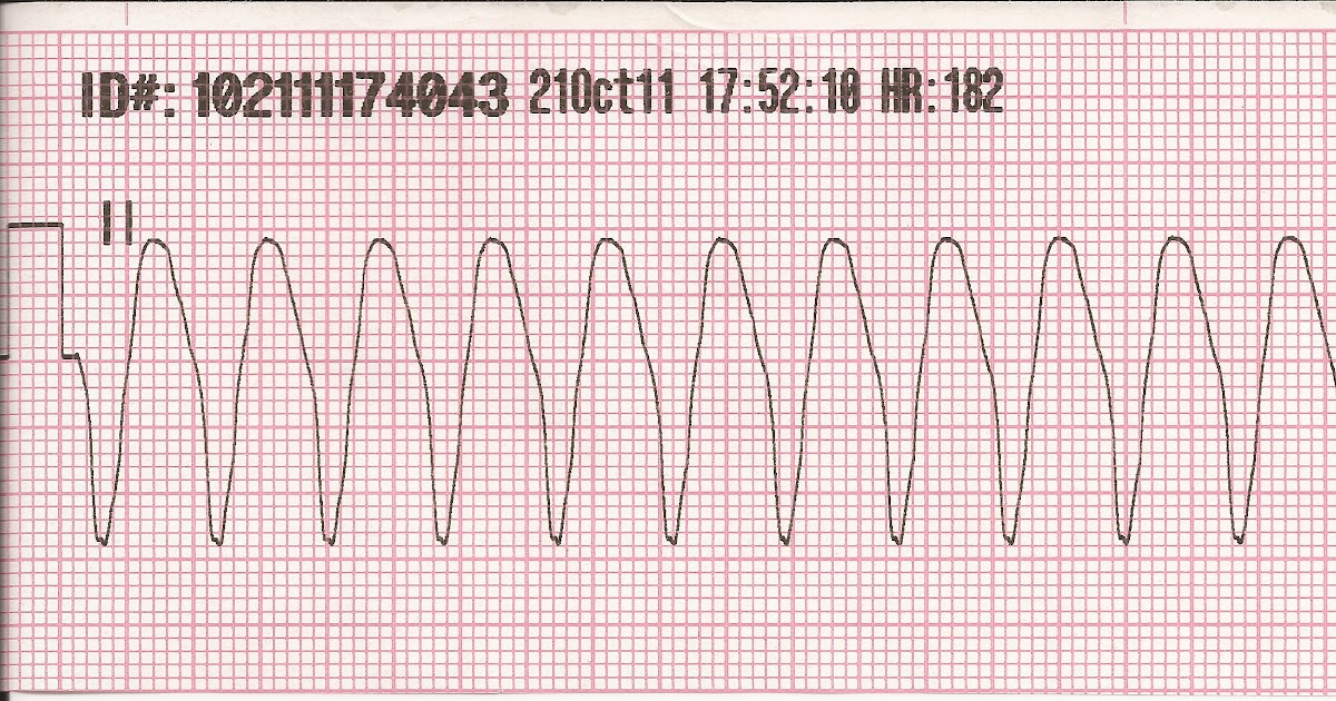
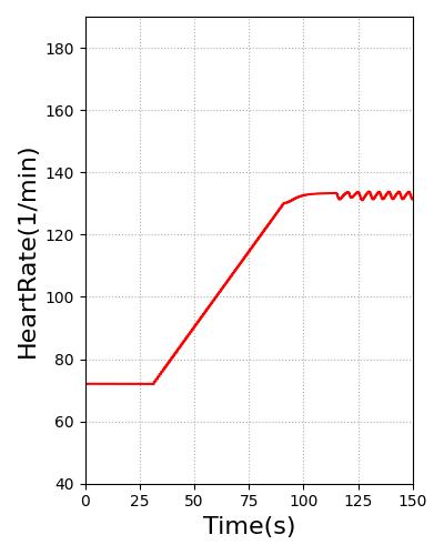
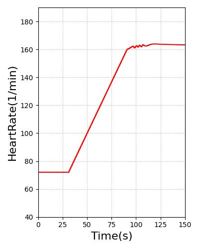
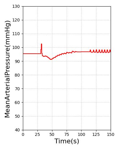
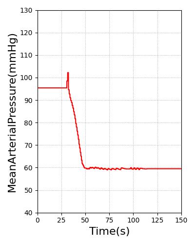
Ventricular tachycardia is defined as either stable or unstable. Stable ventricular tachycardia is characterized by increased heart rate (between 100 and 150) with little change in blood pressure (hemodynamic stability) and an irregular ECG [3] [214]. Unstable ventricular tachycardia is characterized by a heart rate of over 150 [3] with a significant drop in blood pressure (hemodynamic instability) [393] and the ventricular tachycardic ECG waveform.

Figure 12. This ventricular tachycardia ECG waveform is used for both stable and unstable types and is scaled to the heart rate.

Pulse will transition the patient to this heart rate over 60s. For stable ventricular tachycardia, the heart rate baseline is set to 130. For unstable ventricular tachycardia, the heart rate baseline is set to 160. The blood pressure was reduced through for unstable ventricular tachycardia by adding systemic compliance and resistance modifiers. The heart rate and blood pressure for stable and unstable ventricular tachycardia are shown in Figure 13. All feedback and imapcts from additional actions will still impact the hemodynamics of the cardiovascular system from this new starting rate.

Figure 13. Heart rate for stable (Far Left) and unstable ventricular (Middle Left) tachycardia meets the validation of 100-150 and greater than 150, respectively [3]. Stable ventricular (Middle Right) tachycardia shows hemodynamic stability, while hemodynamic instability is present in unstable ventricular tachycardia (Far Right) [214] [393].

Pulseless ventricular tachycardia are characterized by organized electrical activity of the heart, but no mechanical function [5]. The ECG is set to a ventricular tachycardia rhythm for pulseless ventricular tacycardia; however, the amplitude of the waveform is reduced to reflect the weaker electrical activity [5]. All feedback and imapcts from additional actions will NOT impact the hemodynamics of the cardiovascular system, as there is no hemodynamic activity during this arrhythmia.

Hemorrhage

A hemorrhage is a significant reduction in blood volume, which triggers a physiologic response to stabilize cardiovascular function. Hypovolemia is any loss in blood volume, where a loss of more than 35% is considered hypovolemic shock. Hemorrhage causes a reduction in filling pressure for the circulation, leading to a decrease in venous return. This is evidenced by the decrease in mean arterial pressure and cardiac output. If these physiologic values continue to drop, hemorrhagic or hypovolemic shock will occur. There are three stages of shock: a nonprogressive stage, which the normal circulatory responses will lead to a recovery; a progressive stage, which leads to progressively worsening condition and eventual death without intervention; and an irreversible stage, which leads to death regardless of intervention. The sympathetic response is triggered by the decrease in mean arterial blood pressure, specifically by causing the stretch receptors (baroreceptors) to activate. This response triggers an increase in systemic vascular resistance, heart rate, and a decrease in venous compliance. This is discussed in detail in the Nervous Methodology.

Hemorrhage can be intiated in the engine through two methods. The first method allows the user to characterize the hemorrhage by specifying the location (compartment) and bleed rate. Multiple hemorrhages can be applied to a single compartment or to multiple compartments. The user specifies a cardiovascular compartment to apply a hemorrhage. After the hemorrhage has been specified, the total loss rate is the sum of each individual bleed rate to that compartment. This value is set as a negative flow source. This results in a decrease in total blood volume that is linearly proportional to the total loss rate. This flow rate will remain constant throughout the computation. As the blood volume decreases, the blood flow to each compartment will begin to decrease. This could lead to an invalid flow rate for the compartment over time. A second method for specifying hemorrhage deals with this issue. A hemorrhage can also be characterized by specifying the location (compartment) and a severity. The severity is specified with a value between 0 and 1. A path is added to the cardiovascular circuit, but instead of specifying a negative flow rate, a resistance is specified on the path. This provides a calculated flow rate that will increase and decrease based on the dynamic physics of the circuit. This will prevent the insufficient blood flow/volume errors that can occur if the flow rate is not manually managed. When a hemorrhage is initiated with a severity, a minimum and maximum resistance are calculated to bound the severity, as shown in Equations 3 and 4, respectively.

$R_{\min} = (P-P_{T})/cQ$

Equation 3.

Where R_min is the minimum resistance, P is the blood pressure at the compartment hemorrhaging, P_T is the pressure at the hemorrhage flow outlet, Q is the flow through the hemorrhage compartment (not the hemorrhage flow), and c a tuning factor. The tuning factor is employed to ensure a severity of 1.0 corresponds to a hemorrhage rate of approximately 90% of the flow through the compartment. The severity specified in the hemorrhage action is then used to calculate the resistance on the path.

$R_{\max} = (c_{1})*R_{\min}/s$

Equation 4.

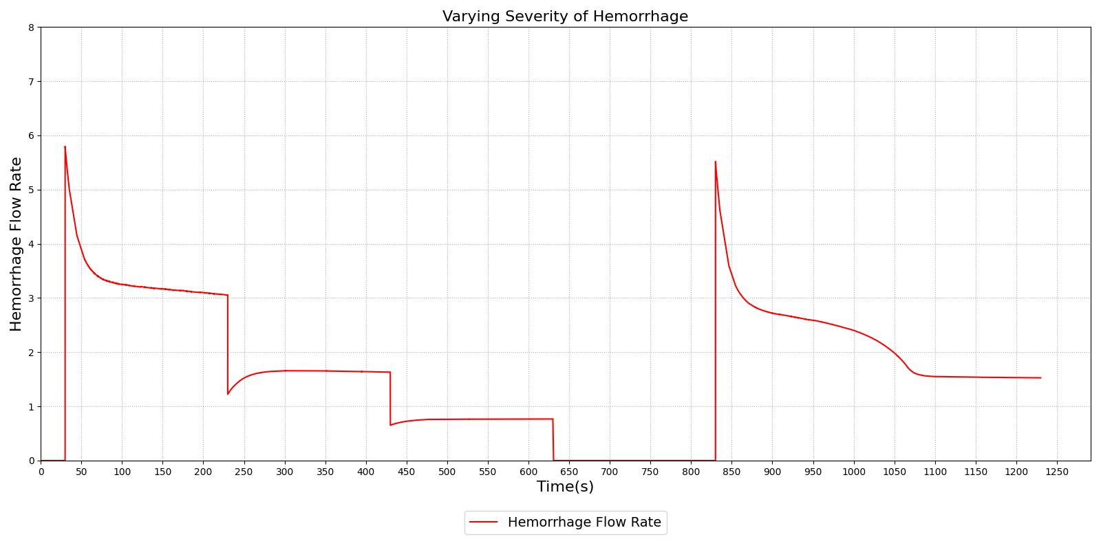
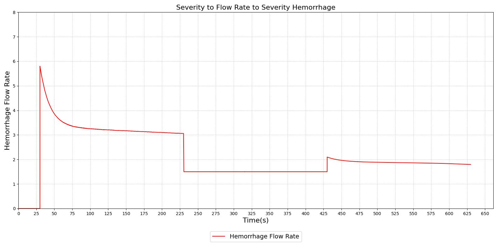
Figure 8 demonstrates the different severity specifications and the impact on the hemorrhage flow rate as the severity is changed or the body responds to the hemorrhage. The results show that the hemorrhage severity changes the flow rate for the hemorrhage as expected, i.e., a 0.5 severity corresponds to 50% of the flow associated with a severity of 1.0. The results also show that as time passes the flow rate will naturally decrease without changing the severity to correspond to the reduction in blood pressure that occurs with hemorrhage. These results also demonstrate the ability to transition from a severity to a flow implementation and back to severity, if required.

Figure 8. Normalized mean arterial pressure and cardiac output as blood loss increases for the Pulse model (left) and the validation data [152] (right).

An internal hemorrhage can also be specified for abdominal cardiovascular compartments, including the aorta, vena cava, stomach, splanchnic, spleen, right and left kidneys, large and small intestines, and liver. The internal hemorrhage allows blood to flow into the abdominal cavity, increasing the pressure in the cavity. For the severity implementation, the hemorrhage outlet compartment is specified as the abdominal cavity for Equation 3. This pressure is applied to the aorta, increasing the localized blood pressure as a result of internal blood accumulation. At this time, the internal hemorrhage is only associated with the abdominal region. In the future, we will add functionality for the brain and lungs (hemothorax).

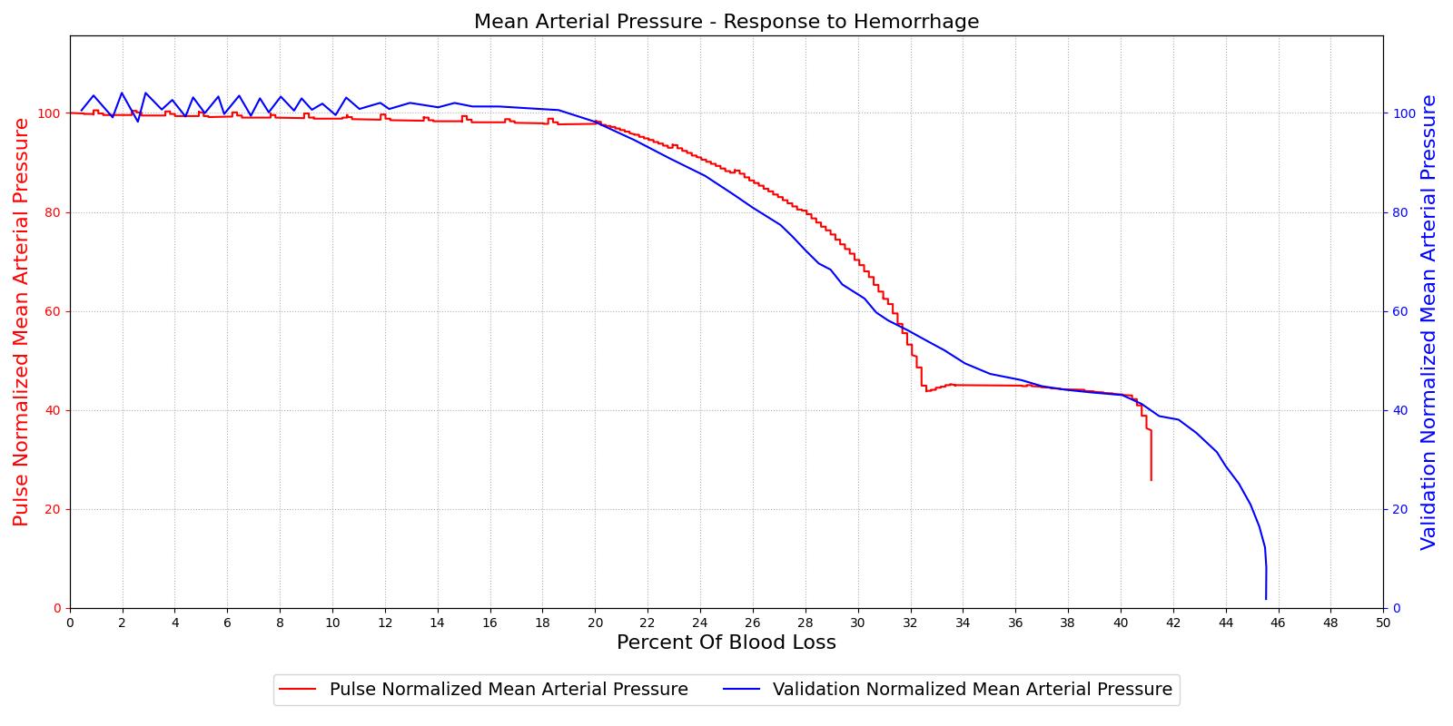
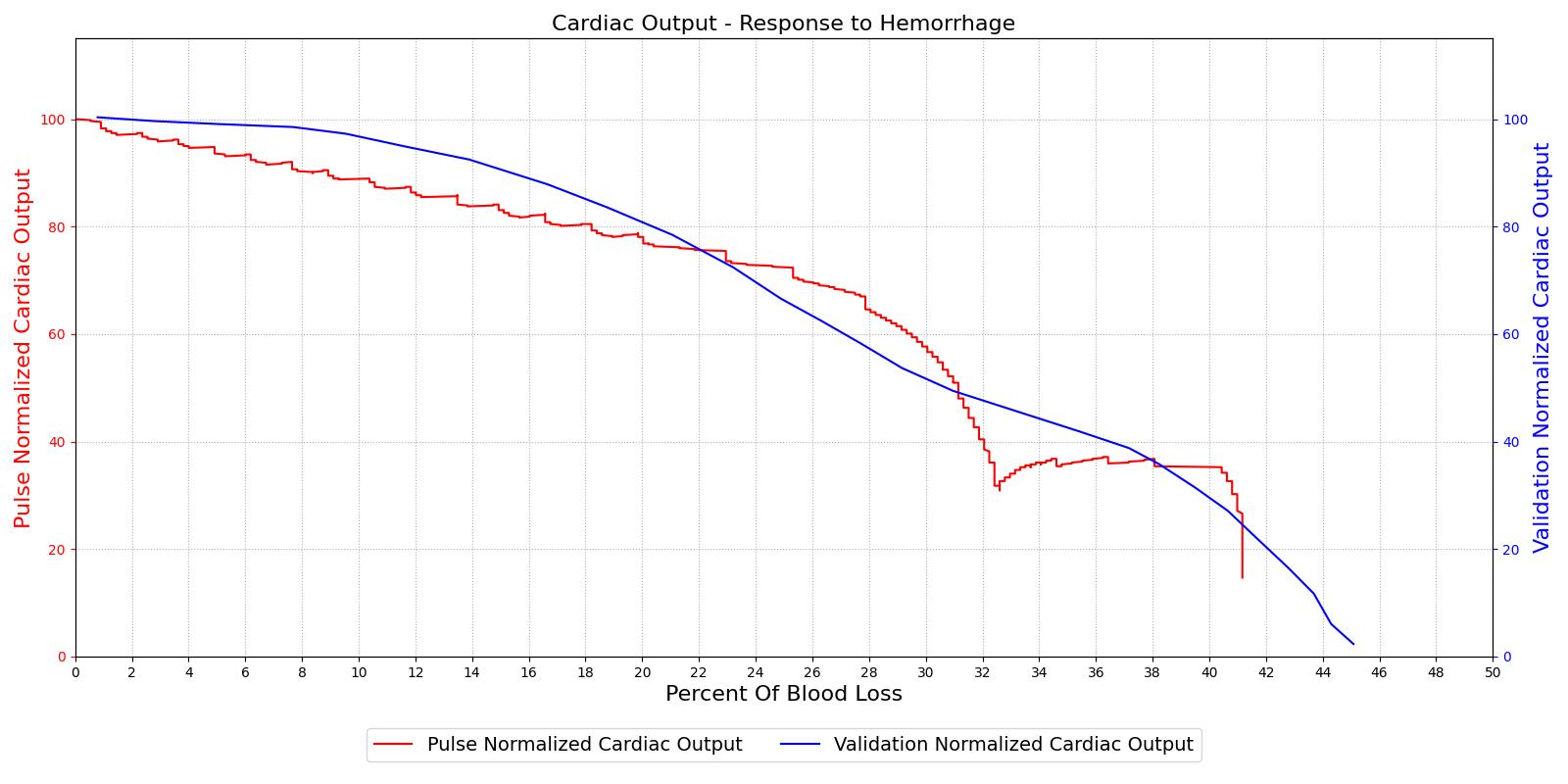
The hemorrhage response was validated with a comparison to the literature. The mean arterial pressure and cardiac output were computed as a function of their baseline value and plotted with the percent blood loss, as shown in Figure 9. The computed results are shown on the left and the validation data [152] is shown on the right.

Figure 9. Normalized mean arterial pressure (left) and cardiac output (right) as blood loss increases for the Pulse model and the validation data [152].

For the hemorrhage to shock scenario, our results maintain MAP through a 20% blood loss and CO begins to slowly decrease as expected. At 20%, we see an approximately linear drop in MAP from a as expected compared to experimental data from [152]. The cardiac output shows the correct trend but a larger error for this region. The "last ditch" plateau is then exhibited from a blood loss of just under 35% to just under 45%. The MAP and CO then drop precipitously as expected.

The different types of shock are evident in the data collected for groups of dogs and published in [152]. Groups I, II, and III show cases of nonprogressive shock, Groups IV, and V show cases of progressive shock, and Group VI is an irreversible shock case. The first three groups recover without intervention, the final case leads quickly to death, and the Group IV and V cases show a short rebound before the physiologic decline that occurs without treatment. These cases were duplicated in the Pulse engine. The results and comparison to validation data are shown in Figure 10.

Figure 10. Normalized mean arterial pressure for different hemorrhage severities to demonstrate the different shock types. The computed Pulse results are on the left and the validation data [152] is on the right.

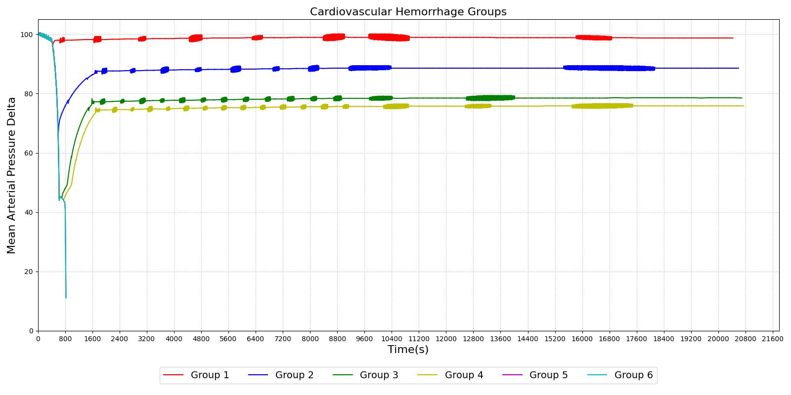
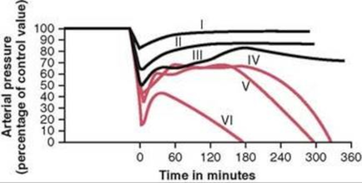
For the first three group hemorrhage scenarios (90%, 65%, and 50% blood loss), if the hemorrhage is arrested the MAP begins to rise and reaches a stable value. However, for the remaining three scenarios, the hemorrhage is unrecoverable for the patient. This is expected compared to the experimental data and for the degree of shock. However, one limitation of the model is that at the turning point between progressive and irreversible shock, the expected behavior is a temporary recovery lasting minutes to hours followed by deterioration and death. The current model has no ability to reverse the curve once the final deterioration toward deaths occurs. This is triggered at a blood pressure of approximately 40-45 mmHg. While the outcome is the same, the short recovery is not captured. Future work will incorporate this improvement.

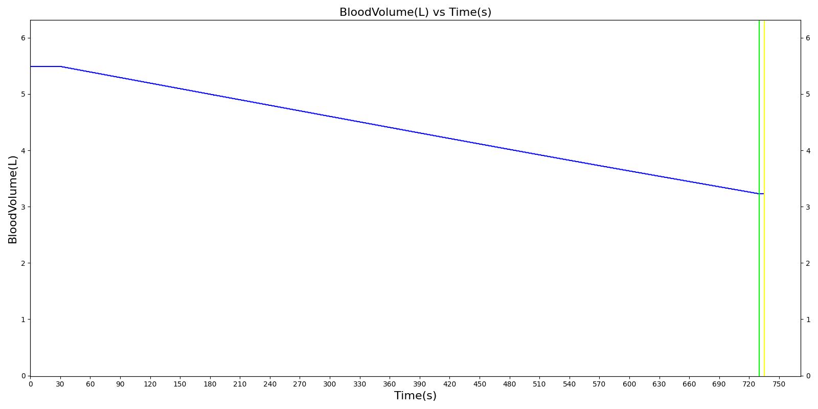
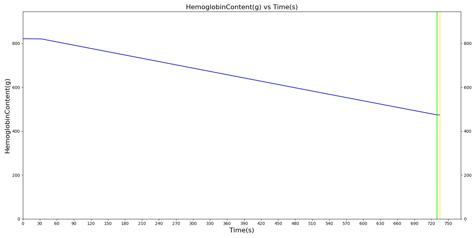
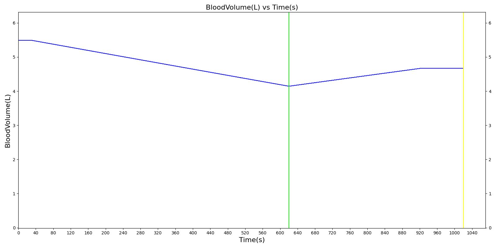
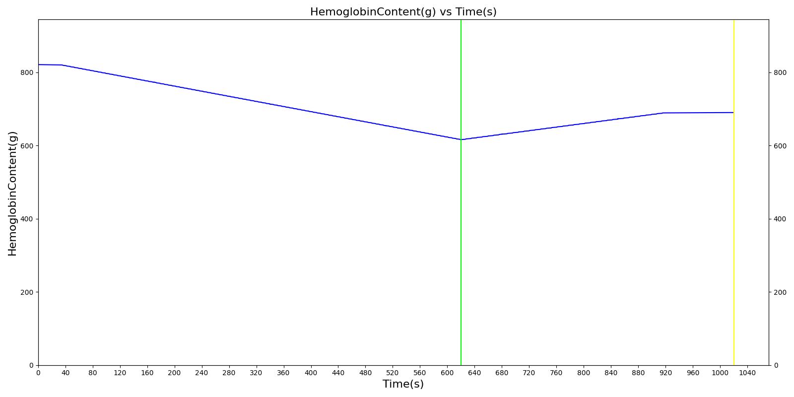
We also saw the expected blood volume, pressure, heart rate, and substance concentration values follow expected trends for the fluid resuscitation scenarios. Figures 11 and 12 show the appropriate substance behavior coupled with the blood volume changes. Like blood volume, the decrease in the substance will be linearly proportional to the bleed rate. For more specific information regarding these substances and their loss due to bleeding, see Blood Chemistry Methodology and Substance Transport Methodology. Figure 11 shows the blood volume and hemoglobin content before, during, and after a massive hemorrhage event with no intervention other than the cessation of hemorrhage. Figure 12 shows a hemorrhage event with subsequent saline administration. Note that the hemoglobin content remains diminished as the blood volume recovers with IV saline. By comparison, Figure 14 shows a blood-product intervention following a hemorrhage event. In that figure, the hemoglobin increases with the blood infusion.

Figure 11. Blood volume and hemoglobin content before, during, and after a massive hemorrhage event with no subsequent intervention.

Figure 12. Blood volume and hemoglobin content before, during, and after a massive hemorrhage event with a subsequent infusion of saline.

Pericardial Effusion

The pericardial effusion action is used to model acute pericardial effusion by adding a flow source on the pericardium. This action leads to a volume accumulation over the course of the simulation. The accumulated volume is used to calculate a pressure source that is applied to the left and right heart. This pressure source is identical to the one used in the pericardial effusion condition. For the pericardial effusion action, the strain-rate dependent compliance of the pericardium is modeled so that the change in intrapericardial pressure is a function of flow rate and the current volume of the pericardium [312].

Interventions

Cardiopulmonary Resuscitation (CPR)

CPR can be preformed to maintain some perfusion through an induced arrhythmia action. The American Heart Association recommends performing chest compressions at a rate of 100-120 per minute with enough force to achieve a chest-compression depth of 5 cm [110]. Gruben et al estimated a required force of approximately 400 N to achieve the required depth [147]. Kim et al found that stroke volumes of 12-35 mL and an effective cardiac output of 1200-3500 mL/min could be achieved with the proper compression technique. The aforementioned hemodynamics are accompanied by an increase in systolic and diastolic pressures and, by extension, mean arterial pressure [197].

Chest compressions are simulated in the engine by adjusting the value of the pressure source that is connected between the common equipotential node and the capacitors that represent the right and left cardiac compliances. The pressure source represents the intrathoracic pressure, thus a positive pressure value represents an increase in intrathoracic pressure. The pressure on the source is calculated from the input force and the biometrics of the patient.

The CPR force of compression can be expressed to the engine in one of two ways, as a Force (ex. N), or depth between 0 and 6 cm, where 6m provides the maximum pressure of 550 N based on the work of Arbogast et al [15]. Pulse provides several actions to prescribe chest compressions:

An instantaneous action: This action allows a user to explicitly set the applied force at the time of the CPR compression call. The provided pressure is maintained in the engine until the next action is provided. Successive compressions are achieved by calling a CPR compression at a desired force, calling for an advance in simulation time, and then calling the next desired force. In this way, the shape of the time-dependent force curve is explicitly set by the user. This action is primarily intended to be used in conjuction with hardware sensors providing Pulse continuous force information.
A single compression action: This action allows users to supply the force to be applied over a specified time. When the compression is applied in Pulse, the evolution of the force is a curve applied over the provided compression time automatically by the engine. A bell shaped force curve is used in accordance with [347]. Once the compression is complete, you must provide another action to keep performing CPR. Users will need to advance time without a compression action to simulate the wait time between compressions.
An automatic compression action: This action allows a user to prescribe a compression frequency to be continuously applied. This will continuously applying compressions at a fixed interval unitl a force or frequency of 0 is provided. A compression duration is derived from the provide frequency. To specify a wait time between compressions, the AppliedForceFraction parameter will inform the engine how much of the derived compression duration to apply the force curve. The remaining time of the compression will have 0 force. For example, a frequecy of 120 bpm will result in a compression duration of 0.5s. An AppliedForceFraction of 0.8, will result in the force curve being applied over 0.4s and 0 force being applie for 0.1s, then the next compression will begin.

The compression-only CPR in the engine is consistent with AHA guidelines for lay rescuer adult CPR [163]. The addition of rescue breathing for health-care provider CPR can be provided using a Bag Valve Mask action.

Hemorrhage Cessation

A “tourniquet” may be applied to a bleeding distal portion of the body to reduce blood flow entering that portion and effectively stopping the bleeding. With the bleeding managed, vital signs should return to their normal state after a sufficient period of time. A “tourniquet” may be simulated in the engine by reducing the bleeding rate associated with a specified hemorrhage. If the hemorrhage leads to significant blood loss, reducing the bleeding rate of that hemorrhage will lead to a return of the arterial pressures as the effect of the baroreceptor response is not outweighed by blood loss. As the MAP increases, heart rate will begin to decrease in proportion to the error control dictated by the baroreceptor reflex. Lastly, cardiac output will begin to increase to a new, stabilized value associated with the new total blood volume.

Intravenous Fluid Administration

Intravenous fluid administration is a continual injection of a compatible fluid into the veins of a patient that has suffered from fluid loss. Due to increasing volume from intravenous fluid administration, blood volume and arterial pressures will increase. Stroke volume will increase due to increased venous return, which will cause an increase in cardiac output. The baroreceptor response will lead to a decrease in the heart rate.

Intravenous fluid administration is simulated by applying a flow source to the vena cava. The flow source and duration of the administration is dictated by the user in the form of a flow rate and IV bag volume. This results in an increase in total blood volume, heart stroke volume, cardiac output, and arterial pressures. Due to increasing arterial pressures, the baroreceptor reflex will begin to decrease heart rate according to the error between the mean arterial pressure and its set point. Additional effects may occur depending on the type of fluid administered. Currently, the user may administer blood, saline, and/or packed red blood cells. Each of these fluids is considered a compound substance with multiple substance components. Further information on the effect of substances during fluid administration can be found in Substance Transport Methodology.

Exacerbations

The pulmonary shunt condition has an exacerbation actions defined to allow for increased/decreased severities during runtime. This exacerbation action will instantaneously (i.e., during the simulation/scenario runtime) change the value of the pulmonary shunt (right, left, or both), based on the severity provided. Exacerbations can either degrade or improve the patient's current condition.

Events

Cardiac Arrest

Cardiac Arrest is a condition in which the pumping of the heart is no longer effective [263]. The Cardiac Arrest event can be triggered by different arrhythmias in the engine. In the current version of the engine, any rhythm associated with a cessation of mechanical function of the heart will trigger a cardiac arrest event. We do not have a defibrillate action at this time. To recover from a cardiac arrest event, the user can change the arrhythmia back to a sinus rhythm. It is also possible to maintain some perfusion by performing chest compressions (see CPR).

Cardiovascular Collapse

Cardiovascular collapse occurs when the blood pressure is no longer sufficient to maintain "open" blood vessels. They "collapse" meaning blood can no longer flow through the vessels. This is generally associated with shock, the vascular tone and blood pressure are no longer sufficient to maintain blood flow [152]. This occurs at at mean arterial pressure of 20 mmHg or lower in the engine. At this time, we do not enforce an irreversible state (stop engine calculation); however, the patient generally does not recover from this, particularly in the presence of shock.

Cardiogenic Shock

In general, the term "shock" refers to inadequate perfusion of the tissues. The several categories of shock serve to signify the origin of the disturbance. Cardiogenic shock is inadequate perfusion due a reduction in the pumping capability of the heart. In the engine, the Cardiogenic Shock event is activated when the cardiac index () is below 2.2 (L/min-m^2) and the systolic blood pressure is less than 90.0 (mmHg) and the pulmonary capillary wedge pressure is greater than 15.0 (mmHg) [81].

Hypovolemic Shock

Hypovolemia is any reduction in blood volume. Hypovolemic shock is defined as a reduction in total blood volume by 35 percent [152]. Typically, this is classified by elevated heart rate and decreased arterial pressure. In the engine, hypovolemia is triggered during a hemorrhage when blood volume has fallen below 65 percent of its normal value.

Results and Conclusions

The Cardiovascular System was validated quantitatively and qualitatively under resting physiologic conditions and transient (action-induced) conditions. The validation is specified with a color coding system, with green indicating good agreement with trends/values, yellow indicating moderate agreement with trends/values, and shades red indicating poor agreement with trends/values.

Validation - Resting Physiologic State

Validation results for system and compartment quantities are listed in Tables 1 and 2. System-level quantities show favorable agreement with validation values. Heart rate, arterial pressures, blood volume, heart stroke volume, and cardiac output are the predominant CV System quantities. These values agree, on average, within ~8 percent of the expected values for the healthy standard patient.

Table 1. Validation of the resting physiologic state comparison of system-level outputs from the engine to referenced values. System-level outputs show favorable agreement with validation data.

Standard Male

Property Name	Expected Value	Engine Value	Percent Error	Notes
BloodVolume(mL)	5518 [152]	Mean of 5491	0.5%
CardiacIndex(L/min_m^2)	2.8 [152]	Mean of 2.9	1.8%	The normal human weighing 70kg has a body surface area of about 1.7 square meteres.
CardiacOutput(mL/min)	5600 [152]	Mean of 5788	3.4%
CerebralBloodFlow(mL/min)	672 [378]	Mean of 681	1.3%
CerebralPerfusionPressure(mmHg)	[60.0,98.0]	Mean of 86.2	0.0%
CoronaryPerfusionPressure(mmHg)	[60.0,80.0] [9]	Mean of 67.66093444824219	0.0%
DiastolicArterialPressure(mmHg)	[60.0,90.0] [383]	Mean of 73.6	0.0%
DiastolicLeftHeartPressure(mmHg)	[4.0,12.0] [96]	Mean of 5.9	0.0%
DiastolicRightHeartPressure(mmHg)	[2.0,8.0] [96]	Mean of 1.8	10.0%
HeartEjectionFraction	0.55 [152]	Mean of 0.57	2.9%
HeartRate(1/min)	[60,100] [238]	Mean of 72	0.0%
HeartStrokeVolume(mL)	[55.3,93.1] [41]	Mean of 80.4	0.0%
IntracranialPressure(mmHg)	[7.0,15.0] [349]	Mean of 9.1	0.0%	Assumes supine adult
MeanArterialPressure(mmHg)	[70.0,105.0] [383]	Mean of 95.3	0.0%
MeanCentralVenousPressure(mmHg)	[2.0,6.0] [383]	Mean of 4.7	0.0%
MeanSkinFlow(mL/s)	4.7 [378]	Mean of 4.7	1.3%
PeripheralPerfusionIndex	[0.029,0.062] [330]	Mean of 0.043	0.0%
PulmonaryCapillariesWedgePressure(mmHg)	[4.0,12.0] [383]	Mean of 6.5	0.0%
PulmonaryDiastolicArterialPressure(mmHg)	[4.0,15.0] [383] [96]	Mean of 15.2	1.4%
PulmonaryMeanArterialPressure(mmHg)	[9.0,18.0] [96]	Mean of 17.4	0.0%
PulmonarySystolicArterialPressure(mmHg)	[15.0,30.0] [383]	Mean of 19.5	0.0%
PulmonaryVascularResistance(mmHg_s/mL)	0.140 [152]	Mean of 0.113	19.3%
PulmonaryVascularResistanceIndex(mmHg_s/mL_m^2)	0.240 [152]	Mean of 0.223	7.1%	The normal human weighing 70kg has a body surface area of about 1.7 square meteres. Therefore, 0.14*1.7.
PulsePressure(mmHg)	[25.0,100.0] [173]	Mean of 40.7	0.0%	SystolicArterialPressure - DiastolicArteralPressure
SystemicVascularResistance(mmHg_s/mL)	1.0 [152]	Mean of 0.9	6.1%
SystolicArterialPressure(mmHg)	[100.0,140.0] [383]	Mean of 114.3	0.0%
SystolicLeftHeartPressure(mmHg)	[100.0,140.0] [174]	Mean of 136.6	0.0%
SystolicRightHeartPressure(mmHg)	[15.0,30.0] [96]	Mean of 32.3	7.7%
TotalPulmonaryPerfusion(mL/min)	[5320.0,5600.0] [152]	Mean of 5645.5	0.8%	[Cardiac Output - 5% Shunt, Cariac Output]

Standard Female

Property Name	Expected Value	Engine Value	Percent Error	Notes
BloodVolume(mL)	4197 [152]	Mean of 4182	0.4%
CardiacIndex(L/min_m^2)	3.0 [152]	Mean of 3.2	6.6%	The normal human weighing 70kg has a body surface area of about 1.7 square meteres.
CardiacOutput(mL/min)	4900 [152]	Mean of 5152	5.1%
CerebralBloodFlow(mL/min)	588 [378]	Mean of 602	2.4%
CerebralPerfusionPressure(mmHg)	[60.0,98.0]	Mean of 86.1	0.0%
CoronaryPerfusionPressure(mmHg)	[60.0,80.0] [9]	Mean of 68.100830078125	0.0%
DiastolicArterialPressure(mmHg)	[60.0,90.0] [383]	Mean of 73.7	0.0%
DiastolicLeftHeartPressure(mmHg)	[4.0,12.0] [96]	Mean of 5.6	0.0%
DiastolicRightHeartPressure(mmHg)	[2.0,8.0] [96]	Mean of 1.8	11.5%
HeartEjectionFraction	0.55 [152]	Mean of 0.55	0.4%
HeartRate(1/min)	[60,100] [238]	Mean of 72	0.0%
HeartStrokeVolume(mL)	[55.3,93.1] [41]	Mean of 71.6	0.0%
IntracranialPressure(mmHg)	[7.0,15.0] [349]	Mean of 9.0	0.0%	Assumes supine adult
MeanArterialPressure(mmHg)	[70.0,105.0] [383]	Mean of 95.2	0.0%
MeanCentralVenousPressure(mmHg)	[2.0,6.0] [383]	Mean of 4.7	0.0%
MeanSkinFlow(mL/s)	4.1 [378]	Mean of 4.2	2.4%
PeripheralPerfusionIndex	[0.029,0.062] [330]	Mean of 0.066	7.2%
PulmonaryCapillariesWedgePressure(mmHg)	[4.0,12.0] [383]	Mean of 6.1	0.0%
PulmonaryDiastolicArterialPressure(mmHg)	[4.0,15.0] [383] [96]	Mean of 14.7	0.0%
PulmonaryMeanArterialPressure(mmHg)	[9.0,18.0] [96]	Mean of 17.2	0.0%
PulmonarySystolicArterialPressure(mmHg)	[15.0,30.0] [383]	Mean of 19.6	0.0%
PulmonaryVascularResistance(mmHg_s/mL)	0.140 [152]	Mean of 0.129	7.5%
PulmonaryVascularResistanceIndex(mmHg_s/mL_m^2)	0.240 [152]	Mean of 0.211	12.1%	The normal human weighing 70kg has a body surface area of about 1.7 square meteres. Therefore, 0.14*1.7.
PulsePressure(mmHg)	[25.0,100.0] [173]	Mean of 40.8	0.0%	SystolicArterialPressure - DiastolicArteralPressure
SystemicVascularResistance(mmHg_s/mL)	1.0 [152]	Mean of 1.1	5.4%
SystolicArterialPressure(mmHg)	[100.0,140.0] [383]	Mean of 114.4	0.0%
SystolicLeftHeartPressure(mmHg)	[100.0,140.0] [174]	Mean of 136.1	0.0%
SystolicRightHeartPressure(mmHg)	[15.0,30.0] [96]	Mean of 32.1	6.9%
TotalPulmonaryPerfusion(mL/min)	[5320.0,5600.0] [152]	Mean of 5025.6	5.5%	[Cardiac Output - 5% Shunt, Cariac Output]

Table 2. Validation of the resting physiologic state comparison of compartment-level outputs from the engine to referenced values. The compartments are currently validated on a flow/volume basis. Flows and most of the volumes show good agreement with validation values.

Standard Male

Property Name	Expected Value	Engine Value	Percent Error
Aorta-Volume(mL)	275.9 [378]	Mean of 286.5	3.9%
Aorta-InFlow(mL/s)	93.3 [378]	Mean of 95.8	2.6%
BrainVasculature-Volume(mL)	66.2 [378]	Mean of 68.4	3.3%
BrainVasculature-InFlow(mL/s)	11.2 [378]	Mean of 11.3	1.3%
BrainVasculature-Oxygen-PartialPressure(mmHg)	40.0 [82]	Mean of 39.0	2.6%
BoneVasculature-Volume(mL)	386.2 [378]	Mean of 391.3	1.3%
BoneVasculature-InFlow(mL/s)	4.7 [378]	Mean of 4.7	0.1%
FatVasculature-Volume(mL)	275.9 [378]	Mean of 279.8	1.4%
FatVasculature-InFlow(mL/s)	4.7 [378]	Mean of 4.7	0.1%
KidneyVasculature-Volume(mL)	110.4 [378]	Mean of 103.7	6.0%
KidneyVasculature-InFlow(mL/s)	17.7 [378]	Mean of 17.5	1.4%
LargeIntestineVasculature-Volume(mL)	121.4 [378]	Mean of 123.1	1.4%
LargeIntestineVasculature-InFlow(mL/s)	3.7 [378]	Mean of 3.6	3.0%
LeftArmVasculature-Volume(mL)	110.4 [378]	Mean of 105.4	4.5%
LeftArmVasculature-InFlow(mL/s)	1.4 [378]	Mean of 1.284621238708496	8.2%
LeftHeart-Volume(mL)	[34.0,66.0] [107]	Minimum of 61.7	0.0%
LeftHeart-Volume(mL)	[131.0,189.0] [107]	Maximum of 142.2	0.0%
LeftHeart-Pressure(mmHg)	[4.0,12.0] [96]	Minimum of 5.8	0.0%
LeftHeart-Pressure(mmHg)	[100.0,140.0] [174]	Maximum of 136.6	0.0%
LeftHeart-InFlow(mL/s)	94.7 [378]	Mean of 96.1	1.5%
LeftKidneyVasculature-Volume(mL)	55.2 [378]	Mean of 51.8	6.0%
LeftKidneyVasculature-InFlow(mL/s)	8.9 [378]	Mean of 8.7	1.4%
LeftLegVasculature-Volume(mL)	220.7 [378]	Mean of 215.5	2.4%
LeftLegVasculature-InFlow(mL/s)	4.9 [172]	Mean of 4.6417694091796875	5.3%
LeftPulmonaryArteries-Volume(mL)	78.6 [378]	Mean of 85.8	9.1%
LeftPulmonaryArteries-InFlow(mL/s)	44.3 [378]	Mean of 47.0	5.9%
LeftPulmonaryCapillaries-Volume(mL)	52.4 [378]	Mean of 56.2	7.2%
LeftPulmonaryCapillaries-InFlow(mL/s)	44.3 [378]	Mean of 45.0	1.4%
LeftPulmonaryVeins-Volume(mL)	144.2 [378]	Mean of 156.9	8.9%
LeftPulmonaryVeins-InFlow(mL/s)	44.3 [378]	Mean of 46.2	4.1%
LiverVasculature-Volume(mL)	551.8 [378]	Mean of 540.5	2.0%
LiverVasculature-InFlow(mL/s)	23.8 [152]	Mean of 22.5	5.3%
MuscleVasculature-Volume(mL)	772.5 [378]	Mean of 737.5	4.5%
MuscleVasculature-InFlow(mL/s)	15.9 [378]	Mean of 14.6	8.2%
MyocardiumVasculature-Volume(mL)	55.2 [378]	Mean of 58.0	5.1%
MyocardiumVasculature-InFlow(mL/s)	3.7 [378]	Mean of 3.9	4.9%
PulmonaryArteries-Volume(mL)	165.5 [378]	Mean of 171.1	3.4%
PulmonaryArteries-InFlow(mL/s)	93.3 [378]	Mean of 96.5	3.4%
PulmonaryArteries-Pressure(mmHg)	[4.0,12.0] [383]	Minimum of 15.2	26.7%
PulmonaryArteries-Pressure(mmHg)	[15.0,30.0] [383]	Maximum of 19.5	0.0%
PulmonaryCapillaries-Volume(mL)	110.4 [378]	Mean of 111.4	0.9%
PulmonaryCapillaries-InFlow(mL/s)	93.3 [378]	Mean of 93.3	0.0%
PulmonaryCapillaries-Pressure(mmHg)	[4.0,12.0] [383]	Mean of 9.5	0.0%
PulmonaryVeins-Volume(mL)	303.5 [378]	Mean of 310.4	2.3%
PulmonaryVeins-InFlow(mL/s)	93.3 [378]	Mean of 96.1	2.9%
PulmonaryVeins-Pressure(mmHg)	[4.0,12.0] [383]	Mean of 6.5	0.0%
RightArmVasculature-Volume(mL)	110.4 [378]	Mean of 105.4	4.5%
RightArmVasculature-InFlow(mL/s)	1.4 [132]	Mean of 1.284621238708496	8.2%
RightHeart-Volume(mL)	[50.0,100.0] [107] [96]	Minimum of 59.8	0.0%
RightHeart-Volume(mL)	[100.0,223.0] [107] [96]	Maximum of 140.3	0.0%
RightHeart-Pressure(mmHg)	[2.0,8.0] [96]	Minimum of 1.8	10.2%
RightHeart-Pressure(mmHg)	[15.0,30.0] [96]	Maximum of 32.3	7.7%
RightHeart-InFlow(mL/s)	94.7 [378]	Mean of 96.6	2.0%
RightKidneyVasculature-Volume(mL)	55.2 [378]	Mean of 51.8	6.0%
RightKidneyVasculature-InFlow(mL/s)	8.9 [378]	Mean of 8.7	1.4%
RightLegVasculature-Volume(mL)	220.7 [378]	Mean of 215.5	2.4%
RightLegVasculature-InFlow(mL/s)	4.9 [172]	Mean of 4.6417694091796875	5.3%
RightPulmonaryArteries-Volume(mL)	86.9 [378]	Mean of 85.3	1.8%
RightPulmonaryArteries-InFlow(mL/s)	49.0 [378]	Mean of 49.6	1.1%
RightPulmonaryCapillaries-Volume(mL)	57.9 [378]	Mean of 55.2	4.7%
RightPulmonaryCapillaries-InFlow(mL/s)	49.0 [378]	Mean of 48.4	1.3%
RightPulmonaryVeins-Volume(mL)	159.3 [378]	Mean of 153.5	3.7%
RightPulmonaryVeins-InFlow(mL/s)	49.0 [378]	Mean of 49.9	1.8%
SkinVasculature-Volume(mL)	165.5 [378]	Mean of 171.0	3.3%
SkinVasculature-InFlow(mL/s)	4.7 [378]	Mean of 4.7	1.3%
SmallIntestineVasculature-Volume(mL)	209.7 [378]	Mean of 212.8	1.5%
SmallIntestineVasculature-InFlow(mL/s)	9.3 [378]	Mean of 8.7	6.8%
SplanchnicVasculature-Volume(mL)	55.2 [378]	Mean of 56.0	1.5%
SplanchnicVasculature-InFlow(mL/s)	0.9 [378]	Mean of 1.0	9.9%
SpleenVasculature-Volume(mL)	77.2 [378]	Mean of 80.3	4.0%
SpleenVasculature-InFlow(mL/s)	2.8 [378]	Mean of 3.0	5.6%
VenaCava-Volume(mL)	965.6 [378]	Mean of 942.1	2.4%
VenaCava-InFlow(mL/s)	93.3 [378]	Mean of 95.7	2.6%

Standard Female

Property Name	Expected Value	Engine Value	Percent Error
Aorta-Volume(mL)	209.8 [378]	Mean of 216.2	3.0%
Aorta-InFlow(mL/s)	81.7 [378]	Mean of 85.3	4.5%
BrainVasculature-Volume(mL)	50.4 [378]	Mean of 51.7	2.7%
BrainVasculature-InFlow(mL/s)	9.8 [378]	Mean of 10.0	2.4%
BrainVasculature-Oxygen-PartialPressure(mmHg)	40.0 [82]	Mean of 40.5	1.4%
BoneVasculature-Volume(mL)	293.8 [378]	Mean of 297.0	1.1%
BoneVasculature-InFlow(mL/s)	4.1 [378]	Mean of 4.1	1.0%
FatVasculature-Volume(mL)	356.7 [378]	Mean of 361.0	1.2%
FatVasculature-InFlow(mL/s)	6.9 [378]	Mean of 7.0	1.0%
KidneyVasculature-Volume(mL)	83.9 [378]	Mean of 79.6	5.1%
KidneyVasculature-InFlow(mL/s)	13.9 [378]	Mean of 14.9	7.7%
LargeIntestineVasculature-Volume(mL)	92.3 [378]	Mean of 93.3	1.1%
LargeIntestineVasculature-InFlow(mL/s)	4.1 [378]	Mean of 4.0	1.9%
LeftArmVasculature-Volume(mL)	83.9 [378]	Mean of 80.0	4.7%
LeftArmVasculature-InFlow(mL/s)	1.225 [378]	Mean of 1.1365269422531128	7.2%
LeftHeart-Volume(mL)	[34.0,66.0] [107]	Minimum of 59.0	0.0%
LeftHeart-Volume(mL)	[131.0,189.0] [107]	Maximum of 130.8	0.2%
LeftHeart-Pressure(mmHg)	[4.0,12.0] [96]	Minimum of 5.5	0.0%
LeftHeart-Pressure(mmHg)	[100.0,140.0] [174]	Maximum of 136.2	0.0%
LeftHeart-InFlow(mL/s)	94.7 [378]	Mean of 85.6	9.6%
LeftKidneyVasculature-Volume(mL)	42.0 [378]	Mean of 39.8	5.1%
LeftKidneyVasculature-InFlow(mL/s)	6.9 [378]	Mean of 7.5	7.7%
LeftLegVasculature-Volume(mL)	167.9 [378]	Mean of 163.6	2.6%
LeftLegVasculature-InFlow(mL/s)	4.2875 [172]	Mean of 4.106603145599365	4.2%
LeftPulmonaryArteries-Volume(mL)	59.8 [378]	Mean of 64.6	8.0%
LeftPulmonaryArteries-InFlow(mL/s)	38.8 [378]	Mean of 41.8	7.9%
LeftPulmonaryCapillaries-Volume(mL)	39.9 [378]	Mean of 41.0	2.9%
LeftPulmonaryCapillaries-InFlow(mL/s)	38.8 [378]	Mean of 40.1	3.3%
LeftPulmonaryVeins-Volume(mL)	109.6 [378]	Mean of 110.1	0.5%
LeftPulmonaryVeins-InFlow(mL/s)	38.8 [378]	Mean of 41.1	6.0%
LiverVasculature-Volume(mL)	419.7 [378]	Mean of 410.0	2.3%
LiverVasculature-InFlow(mL/s)	22.1 [152]	Mean of 21.1	4.3%
MuscleVasculature-Volume(mL)	440.7 [378]	Mean of 419.8	4.7%
MuscleVasculature-InFlow(mL/s)	9.8 [378]	Mean of 9.1	7.2%
MyocardiumVasculature-Volume(mL)	42.0 [378]	Mean of 44.0	4.9%
MyocardiumVasculature-InFlow(mL/s)	4.1 [378]	Mean of 4.3	6.1%
PulmonaryArteries-Volume(mL)	125.9 [378]	Mean of 128.7	2.2%
PulmonaryArteries-InFlow(mL/s)	81.7 [378]	Mean of 86.0	5.3%
PulmonaryArteries-Pressure(mmHg)	[4.0,12.0] [383]	Minimum of 14.7	22.6%
PulmonaryArteries-Pressure(mmHg)	[15.0,30.0] [383]	Maximum of 19.7	0.0%
PulmonaryCapillaries-Volume(mL)	83.9 [378]	Mean of 81.1	3.3%
PulmonaryCapillaries-InFlow(mL/s)	81.7 [378]	Mean of 83.2	1.8%
PulmonaryCapillaries-Pressure(mmHg)	[4.0,12.0] [383]	Mean of 9.2	0.0%
PulmonaryVeins-Volume(mL)	230.8 [378]	Mean of 216.7	6.1%
PulmonaryVeins-InFlow(mL/s)	81.7 [378]	Mean of 85.6	4.8%
PulmonaryVeins-Pressure(mmHg)	[4.0,12.0] [383]	Mean of 6.1	0.0%
RightArmVasculature-Volume(mL)	83.9 [378]	Mean of 80.0	4.7%
RightArmVasculature-InFlow(mL/s)	1.225 [132]	Mean of 1.1365269422531128	7.2%
RightHeart-Volume(mL)	[50.0,100.0] [107] [96]	Minimum of 58.2	0.0%
RightHeart-Volume(mL)	[100.0,223.0] [107] [96]	Maximum of 130.0	0.0%
RightHeart-Pressure(mmHg)	[2.0,8.0] [96]	Minimum of 1.8	11.5%
RightHeart-Pressure(mmHg)	[15.0,30.0] [96]	Maximum of 32.1	7.0%
RightHeart-InFlow(mL/s)	94.7 [378]	Mean of 86.0	9.2%
RightKidneyVasculature-Volume(mL)	42.0 [378]	Mean of 39.8	5.1%
RightKidneyVasculature-InFlow(mL/s)	6.9 [378]	Mean of 7.5	7.7%
RightLegVasculature-Volume(mL)	167.9 [378]	Mean of 163.6	2.6%
RightLegVasculature-InFlow(mL/s)	4.2875 [172]	Mean of 4.106603145599365	4.2%
RightPulmonaryArteries-Volume(mL)	66.1 [378]	Mean of 64.1	3.0%
RightPulmonaryArteries-InFlow(mL/s)	42.9 [378]	Mean of 44.2	3.0%
RightPulmonaryCapillaries-Volume(mL)	44.1 [378]	Mean of 40.1	9.0%
RightPulmonaryCapillaries-InFlow(mL/s)	42.9 [378]	Mean of 43.1	0.5%
RightPulmonaryVeins-Volume(mL)	121.2 [378]	Mean of 106.5	12.1%
RightPulmonaryVeins-InFlow(mL/s)	42.9 [378]	Mean of 44.4	3.7%
SkinVasculature-Volume(mL)	125.9 [378]	Mean of 129.3	2.7%
SkinVasculature-InFlow(mL/s)	4.1 [378]	Mean of 4.2	2.4%
SmallIntestineVasculature-Volume(mL)	159.5 [378]	Mean of 161.4	1.2%
SmallIntestineVasculature-InFlow(mL/s)	9.0 [378]	Mean of 8.5	5.8%
SplanchnicVasculature-Volume(mL)	42.0 [378]	Mean of 42.5	1.2%
SplanchnicVasculature-InFlow(mL/s)	0.8 [378]	Mean of 0.9	13.4%
SpleenVasculature-Volume(mL)	58.8 [378]	Mean of 60.9	3.7%
SpleenVasculature-InFlow(mL/s)	2.5 [378]	Mean of 2.6	6.8%
VenaCava-Volume(mL)	734.5 [378]	Mean of 708.4	3.6%
VenaCava-InFlow(mL/s)	81.7 [378]	Mean of 85.3	4.4%

Compartment-level quantities show reasonable agreement with the validation values. All of the flows match the reference values within ~10 percent. The volumes show some moderate differences for a few specific compartments. The aorta compartment volume is much smaller than the validated value. The compliance on this compartment needed to remain low in order to preserve the arterial pressure waveform, which led to less volume than expected. Similarly, the vena cava compliance was set in order to maintain the correct cardiac output and arterial pressures; therefore, its expected volume was limited. The right heart pressures and volumes show some disagreement with the validation data. The minimum values for right heart pressure and volume are much lower than valid ranges. This is due to restriction of unstressed volume in the right heart, which currently has an unstressed volume of zero. An increase in unstressed volume would shift the pressure volume minimums up, while also preserving the maximum values within their respective ranges. The Cardiovascular System is tuned to vitals output validation (Table 1), as well as good agreement with insults' and interventions’ expected trends and values (see the following section). In addition, compartment validation was achieved on a reasonable level.

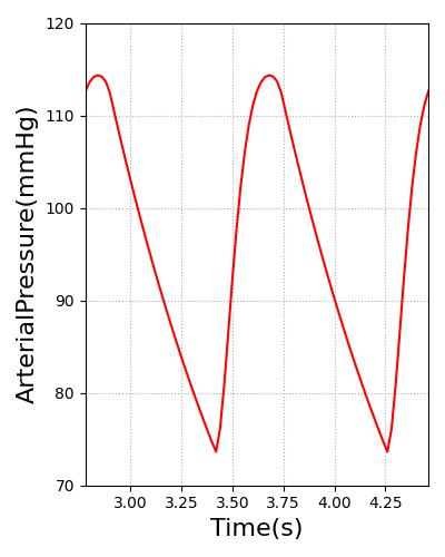
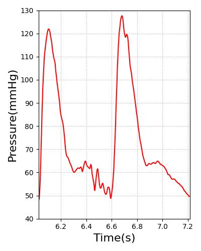
The arterial pressure waveform was validated according to the plot shown in Figure 13. It displays the engine arterial pressure against measured arterial pressure. The diastolic and systolic pressures were validated using data shown in Table 1. To validate the waveform shape and demonstrate the overall feature match of the engine pressure waveform with the validation data, we used a waveform from PhysioNet [137] . However, the patient heart rate and parameters are slightly different than the engine patient. This led to timing discrepancies and differences in the diastolic and systolic pressures. To demonstrate the waveform feature matching, a separate axis is used for each data set. In the future, we may create a patient more representative of the one used for the PhysioNet waveform. This would show both the ability of the engine to model different patients and the pressure waveform feature matching. The shapes of both waveforms match well, showing rapid pressure increases as the heart contraction begins to occur. The main difference in the shape of each plot is the small pressure oscillations that occur after the initial pressure drop in the validation data. This is the dicrotic notch, which occurs from slight flow reversal from the aorta back into the left ventricle before the valves close [357] . This is not currently being modeled in the engine, but improvements in the circuit model, including the addition of inertance and diodes that allow retrograde flow, will likely enable the engine waveform to capture more detail.

Figure 13. Arterial pressure waveform comparisons. The diastolic and systolic pressures were validated using the data shown in Table 1. To validate the waveform shape and demonstrate the overall feature match of the engine pressure waveform with the validation data, a waveform was found on PhysioNet [137] . However, the patient heart rate and parameters are slightly different than the engine patient. This led to timing discrepancies and differences in the diastolic and systolic pressures. To demonstrate the waveform feature matching, a separate axis is used for each data set. Both the validation waveform and the engine waveform show sharp increases in pressure during the systolic period. After the contraction occurs, the pressure begins decreasing and that is where the main difference in the engine and the validation data occur. There is a dip and subsequent rise in the arterial pressure that occurs due to the dicrotic notch, which the engine does not capture.

Validation - Actions and Conditions

All actions in the CV System were validated. A summary of this validation is shown in Table 3. More details on each individual scenario's validation can be found below.

Table 3. Cumulative validation results for Cardiovascular specific conditions and actions scenarios.

Key
Good agreement: correct trends or <10% deviation from expected
Some deviation: correct trend and/or <30% deviation from expected
Poor agreement: incorrect trends or >30% deviation from expected

Scenario	Description	Good	Decent	Bad
Arrhythmia - Asystole To NormalSinus	Asystole for 3 min	7	0	0
Arrhythmia - NormalSinus To SinusBradycardia	Bradycardia for 2 min	7	0	0
Arrhythmia - Asystole To SinusBradycardia	Asystole for 2 min	7	0	0
Arrhythmia - NormalSinus To SinusTachycardia	Tachycardia for 2 min	7	0	0
Arrhythmia - Asystole To SinusTachycardia	Asystole for 2 min	7	0	0
Arrhythmia - Sinus Pulseless Electrical Activity To NormalSinus	PEA for 3 min	7	0	0
Arrhythmia - Coarse Ventricular Fibrillation To NormalSinus	Coarse VFIB for 3 min	7	0	0
Arrhythmia - Fine Ventricular Fibrillation To NormalSinus	Fine VFIB for 3 min	7	0	0
Arrhythmia - NormalSinus To Stable Ventricular Tachycardia	Stable VTACH for 2 min	7	0	0
Arrhythmia - Asystole To Stable Ventricular Tachycardia	Asystole for 2 min	7	0	0
Arrhythmia - NormalSinus To Unstable Ventricular Tachycardia	Unstable VTACH for 2 min	6	0	1
Arrhythmia - Asystole To Unstable Ventricular Tachycardia	Asystole for 2 min	6	0	1
Arrhythmia - Pulseless Ventricular Tachycardia To NormalSinus	Pulseless VTACH for 3 min	7	0	0
CPR	Cardiac arrest is initiated, and CPR is performed.	22	2	0
Hemorrhage Class 1 - Femoral	15% hemorrhage from femoral artery	13	1	0
Hemorrhage Class 2 - Brachial	25% hemorrhage from right arm	12	2	0
Hemorrhage Class 2 - Blood	25% hemorrhage then intravenous whole blood administration	14	0	0
Hemorrhage Class 2 - Spleen	25% hemorrhage from spleen - internal hemorrhage	14	0	0
Hemorrhage Class 2 - Saline	25% hemorrhage then intravenous saline administration	21	0	0
Hemorrhage Class 3 - No Fluids	35% hemorrhage	13	0	1
Hemorrhage Class 3 - RBC	30% hemorrhage then packed red blood cell administration	19	1	1
Hemorrhage to Shock	Hemorrhage until death	13	0	1
Pericardial Effusion - Chronic	Patient has an effused pericardium with an accumulated volume of 500 ml.	9	0	0
Pericardial Effusion - Acute	Pericardium volume starts at 500mL and increases at 6 mL/min.	17	1	0
	Total	256	7	5

Arrhythmia

There are 13 scenarios for arrhythmia validation. Each arrhythmia is validated in its own scenario. Each scenario starts with a stabilized patient in normal sinus, enter an arrhythmia for several minutes, then returns to normal sinus. Several additional scenarios test going to asystole and returning to each of the active (non pulseless) cardiac rhythms.

Asystole

Table 3. Validation matrix for going from normal sinus, to asystole, back to normal sinus. The table shows the engine output compared to key hemodynamic and respiratory parameters.

Asystole To NormalSinus	Notes	Occurrence Time (s)	Sample Scenario Time (s)	Heart Rate (beats/min)	Mean Arterial Pressure (mmHg)	Coronary Perfusion Pressure (mmHg)	Oxygen Saturation (mmHg)	Cardiac Output(mL/min)	Stroke Volume (mL)	ECG Output (mV)
Asystole		30	180	0 [2]	18 +/- 11 [280], Significant drop [20], 33 +/- 10 [197]	13.4 +/- 8.5 [279]	Will decrease as HR and RR stay at 0	0 [2]	0 [2]	Flatline/Asystole [2]
Normal Sinus		210	300	Return to normal after period of recovery	Return to normal after period of recovery	Return to normal after period of recovery	Return to normal after period of recovery	Return to normal after period of recovery	Return to normal after period of recovery	Normal Sinus [2]

Sinus Bradycardia

Table 4. Validation matrix for going from nornal sinus, to sinus bradycardia, back to normal sinus. The table shows the engine output compared to key hemodynamic and respiratory parameters.

NormalSinus To SinusBradycardia	Notes	Occurrence Time (s)	Sample Scenario Time (s)	Heart Rate (beats/min)	Mean Arterial Pressure (mmHg)	Coronary Perfusion Pressure (mmHg)	Oxygen Saturation (mmHg)	Cardiac Output(mL/min)	Stroke Volume (mL)	ECG Output (mV)
Sinus Bradycardia		30	130	Between 40 and 60 [4]	Decrease [4]	Decrease [4]	Little to no change	Decrease [4]	N/A	Normal Sinus[4]
Normal Sinus		210	300	Return to normal after period of recovery	Return to normal after period of recovery	Return to normal after period of recovery	Return to normal after period of recovery	Return to normal after period of recovery	Return to normal after period of recovery	Normal Sinus [2]

Table 5. Validation matrix form nornal sinus, to asystole, to sinus bradycardia. The table shows the engine output compared to key hemodynamic and respiratory parameters.

Asystole To SinusBradycardia	Notes	Occurrence Time (s)	Sample Scenario Time (s)	Heart Rate (beats/min)	Mean Arterial Pressure (mmHg)	Coronary Perfusion Pressure (mmHg)	Oxygen Saturation (mmHg)	Cardiac Output(mL/min)	Stroke Volume (mL)	ECG Output (mV)
Asystole		30	180	0 [2]	18 +/- 11 [280], Significant drop [20], 33 +/- 10 [197]	13.4 +/- 8.5 [279]	Will decrease as HR and RR stay at 0	0 [2]	0 [2]	Flatline/Asystole [2]
Sinus Bradycardia		30	130	Between 40 and 60 @ACLS2021Bradycardia	Decrease [4]	Decrease [4]	Little to no change	Decrease [4]	N/A	Normal Sinus[4]

Sinus Tachycardia

Table 6. Validation matrix for going from nornal sinus, to sinus tachycardia, back to normal sinus. The table shows the engine output compared to key hemodynamic and respiratory parameters.

NormalSinus To SinusTachycardia	Notes	Action Occurrence Time (s)	Sample Scenario Time (s)	Heart Rate (beats/min)	Mean Arterial Pressure (mmHg)	Coronary Perfusion Pressure (mmHg)	Oxygen Saturation (mmHg)	Cardiac Output(mL/min)	Stroke Volume (mL)	ECG Output (mV)
Sinus Tachycardia		30	130	>100 [3]	Little to no change [214]	Little to no change [214]	Little to no change [214]	Increase [344]	Decreases as Heart Rate increases [19]	Normal Sinus[3]
Normal Sinus		210	300	Return to normal after period of recovery	Return to normal after period of recovery	Return to normal after period of recovery	Return to normal after period of recovery	Return to normal after period of recovery	Return to normal after period of recovery	Normal Sinus [2]

Table 7. Validation matrix for going from nornal sinus, to asystole, to sinus tachycardia. The table shows the engine output compared to key hemodynamic and respiratory parameters.

Asystole To SinusTachycardia	Notes	Occurrence Time (s)	Sample Scenario Time (s)	Heart Rate (beats/min)	Mean Arterial Pressure (mmHg)	Coronary Perfusion Pressure (mmHg)	Oxygen Saturation (mmHg)	Cardiac Output(mL/min)	Stroke Volume (mL)	ECG Output (mV)
Asystole		30	180	0 [2]	18 +/- 11 [280], Significant drop [20], 33 +/- 10 [197]	13.4 +/- 8.5 [279]	Will decrease as HR and RR stay at 0	0 [2]	0 [2]	Flatline/Asystole [2]
Sinus Tachycardia		30	130	>100 [3]	Little to no change [214]	Little to no change [214]	Little to no change [214]	Increase [344]	Decreases as Heart Rate increases [19]	Normal Sinus[3]

Sinus Pulseless Electrical Activity

Table 8. Validation matrix for Sinus Pulseless Electrical Activity. The table shows the engine output compared to key hemodynamic and respiratory parameters

Sinus Pulseless Electrical Activity To NormalSinus	Notes	Occurrence Time (s)	Sample Scenario Time (s)	Heart Rate (beats/min)	Mean Arterial Pressure (mmHg)	Coronary Perfusion Pressure (mmHg)	Oxygen Saturation (mmHg)	Cardiac Output(mL/min)	Stroke Volume (mL)	ECG Output (mV)
SinusPulselessElectricalActivity		30	180	0 [2]	18 +/- 11 [280], Significant drop [20], 33 +/- 10 [197]	13.4 +/- 8.5 [279]	Will decrease as HR and RR stay at 0	0 [2]	0 [2]	Sinus w/ Reduced Amplitude [2]
Normal Sinus		210	300	Return to normal after period of recovery	Return to normal after period of recovery	Return to normal after period of recovery	Return to normal after period of recovery	Return to normal after period of recovery	Return to normal after period of recovery	Normal Sinus [2]

Ventricular Fibrillation

Course and fine ventricular fibrillation only differ by the ECG waveform output. Physiology is modelled identically for both.

Table 9. Validation matrix for going from normal sinus, to coarse Ventricular Fibrillation, back to normal sinus. The table shows the engine output compared to key hemodynamic and respiratory parameters.

Coarse Ventricular Fibrillation To NormalSinus	Notes	Occurrence Time (s)	Sample Scenario Time (s)	Heart Rate (beats/min)	Mean Arterial Pressure (mmHg)	Coronary Perfusion Pressure (mmHg)	Oxygen Saturation (mmHg)	Cardiac Output(mL/min)	Stroke Volume (mL)	ECG Output (mV)
CoarseVentricularFibrillation		30	180	0 [2]	18 +/- 11 [280], Significant drop [20], 33 +/- 10 [197]	13.4 +/- 8.5 [279]	Will decrease as HR and RR stay at 0	0 [2]	0 [2]	Coarse Ventricular Fibrillation [63]
Normal Sinus		210	300	Return to normal after period of recovery	Return to normal after period of recovery	Return to normal after period of recovery	Return to normal after period of recovery	Return to normal after period of recovery	Return to normal after period of recovery	Normal Sinus [2]

Table 10. Validation matrix for going from normal sinus, to fine Ventricular Fibrillation, back to normal sinus. The table shows the engine output compared to key hemodynamic and respiratory parameters.

Fine Ventricular Fibrillation To NormalSinus	Notes	Occurrence Time (s)	Sample Scenario Time (s)	Heart Rate (beats/min)	Mean Arterial Pressure (mmHg)	Coronary Perfusion Pressure (mmHg)	Oxygen Saturation (mmHg)	Cardiac Output(mL/min)	Stroke Volume (mL)	ECG Output (mV)
FineVentricularFibrillation		30	180	0 [2]	18 +/- 11 [280], Significant drop [20], 33 +/- 10 [197]	13.4 +/- 8.5 [279]	Will decrease as HR and RR stay at 0	0 [2]	0 [2]	Fine Ventricular Fibrillation [63]
Normal Sinus		210	300	Return to normal after period of recovery	Return to normal after period of recovery	Return to normal after period of recovery	Return to normal after period of recovery	Return to normal after period of recovery	Return to normal after period of recovery	Normal Sinus [2]

Ventricular Tachycardia

Table 11. Validation matrix for going from normal sinus, to stable Ventricular Tachycardia, back to normal sinus. The table shows the engine output compared to key hemodynamic and respiratory parameters.

NormalSinus To Stable Ventricular Tachycardia	Notes	Occurrence Time (s)	Sample Scenario Time (s)	Heart Rate (beats/min)	Mean Arterial Pressure (mmHg)	Coronary Perfusion Pressure (mmHg)	Oxygen Saturation (mmHg)	Cardiac Output(mL/min)	Stroke Volume (mL)	ECG Output (mV)
Stable Ventricular Tachycardia		30	130	100-150 [3]	Little to no change [214]	Little to no change [214]	Little to no change [214]	Increase [344]	Decreases as Heart Rate increases [19]	Ventricular Tachycardia[3]
Normal Sinus		210	300	Return to normal after period of recovery	Return to normal after period of recovery	Return to normal after period of recovery	Return to normal after period of recovery	Return to normal after period of recovery	Return to normal after period of recovery	Normal Sinus [2]

Table 12. Validation matrix for going from normal sinus, to asystole, to stable Ventricular Tachycardia. The table shows the engine output compared to key hemodynamic and respiratory parameters.

Asystole To Stable Ventricular Tachycardia	Notes	Occurrence Time (s)	Sample Scenario Time (s)	Heart Rate (beats/min)	Mean Arterial Pressure (mmHg)	Coronary Perfusion Pressure (mmHg)	Oxygen Saturation (mmHg)	Cardiac Output(mL/min)	Stroke Volume (mL)	ECG Output (mV)
Asystole		30	180	0 [2]	18 +/- 11 [280], Significant drop [20], 33 +/- 10 [197]	13.4 +/- 8.5 [279]	Will decrease as HR and RR stay at 0	0 [2]	0 [2]	Flatline/Asystole [2]
Stable Ventricular Tachycardia		30	130	100-150 [3]	Little to no change [214]	Little to no change [214]	Little to no change [214]	Increase [344]	Decreases as Heart Rate increases [19]	Ventricular Tachycardia[3]

Table 13. Validation matrix for going from normal sinus, to unstable Ventricular Tachycardia, back to normal sinus. The table shows the engine output compared to key hemodynamic and respiratory parameters.

NormalSinus To Unstable Ventricular Tachycardia	Notes	Occurrence Time (s)	Sample Scenario Time (s)	Heart Rate (beats/min)	Mean Arterial Pressure (mmHg)	Coronary Perfusion Pressure (mmHg)	Oxygen Saturation (mmHg)	Cardiac Output(mL/min)	Stroke Volume (mL)	ECG Output (mV)
Untable Ventricular Tachycardia		30	130	> 150 [3]	Decrease [393]	Decrease [393]	Decrease with reduced hemodynamic stability	Decrease [393]	Decrease [393]	Ventricular Tachycardia w/ reduced amplitude [3]
Normal Sinus		210	300	Return to normal after period of recovery	Return to normal after period of recovery	Return to normal after period of recovery	Return to normal after period of recovery	Return to normal after period of recovery	Return to normal after period of recovery	Normal Sinus [2]

Table 14. Validation matrix for going from normal sinus, to asystole, to unstable Ventricular Tachycardia. The table shows the engine output compared to key hemodynamic and respiratory parameters.

Asystole To Unstable Ventricular Tachycardia	Notes	Occurrence Time (s)	Sample Scenario Time (s)	Heart Rate (beats/min)	Mean Arterial Pressure (mmHg)	Coronary Perfusion Pressure (mmHg)	Oxygen Saturation (mmHg)	Cardiac Output(mL/min)	Stroke Volume (mL)	ECG Output (mV)
Asystole		30	180	0 [2]	18 +/- 11 [280], Significant drop [20], 33 +/- 10 [197]	13.4 +/- 8.5 [279]	Will decrease as HR and RR stay at 0	0 [2]	0 [2]	Flatline/Asystole [2]
Untable Ventricular Tachycardia		30	130	> 150 [3]	Decrease [393]	Decrease [393]	Decrease with reduced hemodynamic stability	Decrease [393]	Decrease [393]	Ventricular Tachycardia w/ reduced amplitude [3]

Pulseless Ventricular Tachycardia

Table 15. Validation matrix for Pulseless Ventricular Tachycardia arrhythmias. The table shows the engine output compared to key hemodynamic and respiratory parameters.

Pulseless Ventricular Tachycardia To NormalSinus	Notes	Occurrence Time (s)	Sample Scenario Time (s)	Heart Rate (beats/min)	Mean Arterial Pressure (mmHg)	Coronary Perfusion Pressure (mmHg)	Oxygen Saturation (mmHg)	Cardiac Output(mL/min)	Stroke Volume (mL)	ECG Output (mV)
PulselessVentricularTachycardia		30	180	undetectable [5]	18 +/- 11 [280], Significant drop [20], 33 +/- 10 [197]	13.4 +/- 8.5 [279]	Will decrease as HR and RR stay at 0	0 [5]	0 [5]	Ventricular Tachycardia w/ Reduced Amplitude [5]
Normal Sinus		210	300	Return to normal after period of recovery	Return to normal after period of recovery	Return to normal after period of recovery	Return to normal after period of recovery	Return to normal after period of recovery	Return to normal after period of recovery	Normal Sinus [2]

Cardiopulmonary Resuscitation (CPR)

There are three CPR scenarios for validation. Each scenario perscribes the same frequency with the 3 different types of Chest compression actions. In each scenario, cardiac arrest is initiated externally. Ten seconds later, compressions begin. In each scenario, the compression rate is set to 80 per minute, and the force is set to 311 N (70 pounds) to match the conditions in [299]. Supplemental literature sources were used to validate outputs not available in [299]. All of the physiological variables were within validation ranges in both scenarios with the exception of mean arterial pressure and ejection fraction. The mean arterial pressure in the engine is slightly higher than expected. This is most likely due to the fact that the intravascular pressures are higher than those reported in [299]. However, the engine pressures are within ranges reported in other references [197] , [147]. The ejection fraction is considerably lower in the engine during CPR than the value reported in [197]. The engine ejection fraction is lower because blood tends to pool in the engine right heart during cardiac arrest. The validation failures that occur right at cardiac arrest are mostly due residual dynamics following asystole in the engine. Errors associated with the cessation of heart function in the engine are a known issue, and resolving this issue is a part of the cardiac arrest recommended improvements discussed below.

Table 13. Validation matrix for cardiopulmonary resuscitation (CPR) validation results. The table shows the engine output compared to validation data for key hemodynamic values.

Notes	Action Occurrence Time (s)	Sampled Scenario Time (s)	Heart Rate(beats/min)	Systolic Pressure (mmHg)	Diastolic Pressure (mmHg)	Mean Arterial Pressure (mmHg)	Cardiac Output (mL/min)	Stroke Volume (mL)	Carotid Artery (Brain) Flow (mL/min)	Ejection Fraction (%)
Cardiac Arrest	30	35	0	N/A	N/A	33 +/- 10 [197]	0	0	Approach 0	0
Chest Compressions	40	165-170	80 per minute [Direct calculation]	39.27 [299] Approx. 70-80 [147] 105 +/- 41 [197]	13.97 [299] Approx. 40 [147] 33 +/- 10 [197]	21.13 [299]	17-27% Normal [197]	19.7 [299] 25 +/- 8 [197]	> 0 during compression (translated from dog study) [325]	34% +/- 16 [197]
Chest CompressionsForce Scale	40	165-170	80 per minute [Direct calculation]	39.27 [299] Approx. 70-80 [147] 105 +/- 41 [197]	13.97 [299] Approx. 40 [147] 33 +/- 10 [197]	21.13 [299]	17-27% Normal [197]	19.7 [299] 25 +/- 8 [197]	> 0 during compression (translated from dog study) [325]	34% +/- 16 [197]

Hemorrhage

The hemorrhage action is tested using several scenarios. The class 2 hemorrhage scenario with blood intravenous (IV) administration begins with a healthy patient. After a few seconds, a hemorrhage action is initiated at a rate of 250 milliliters (mL) per minute. The hemorrhage continues for four minutes before the bleeding rate is reduced to 0 mL per minute. After two minutes, 500 mL of IV blood is administered intravenously over five minutes. The other hemorrhage scenarios are similar but with different subsequent interventions. There are also two multi-compartment hemorrhage scenarios. Figure 14 demonstrates the time-evolution of select data, and the validation results are displayed in Tables 6a-f.

The results show decreases in the systolic pressure and minor increases in the diastolic pressure during the course of the hemorrhage. In response to the decreasing arterial pressures, the baroreceptor response raises the heart rate. The blood volume and hemoglobin content were validated through direct calculation by decreasing blood volume by the bleeding rate multiplied by the time. There is a difference between the computed and simulated blood volume post-hemorrhage due to fluid shift between the intravascular and extravascular space. This shift is evident in the period between cessation of hemorrhage and the start of the infusion (top-left panel of Figure 12).

Following the completion of the hemorrhage, intravenous blood is administered. The validation of this action can be found in the IV Fluid Administration section, with the exception of hemoglobin content. There will be an increase in hemoglobin content directly proportional to the amount of blood added from the IV. This value was calculated directly from the known blood volume in the IV bag and hemoglobin concentration of the blood. The engine matched this calculated value exactly.

Figure 20. The class 2 hemorrhage scenario shows the blood volume decreasing linearly with the constant 250 milliliter per minute bleeding rate. The blood hemoglobin content follows this exact trend. At the conclusion of the bleed, the blood volume and hemoglobin are at a lower value. Five hundred (500) milliliters of blood is then administered intravenously over the course of 5 minutes. Both the blood volume and hemoglobin content increase linearly with this administration.

Table 14. Validation matrix for a class I hemorrhage from the femoral artery. The table shows the engine output compared to key hemodynamic and respiratory parameters.

Segment	Notes	Action Occurrence Time (s)	Sampled Scenario Time (s)	Heart Rate (/min)	Mean Arterial Pressure (mmHg)	Blood Volume (mL)	Cardiac Output (mL/min)	Heart Stroke Volume (mL)	Hemoglobin Content (g)	Respiration Rate (/min)
Initiate 90 ml/min Hemorrhage		30	580	Increase [152]	No Change [152]	4675	No Change @guyton2006medical	Decrease [152]	700	No Change [152]
Stop Hemorrhage		580	980	No Change	No Change	No Change	No Change	No Change	No Change	No Change

Table 15. Validation matrix for a class II hemorrhage from the brachial artery. The table shows the engine output compared to key hemodynamic and respiratory parameters.

Segment	Notes	Action Occurrence Time (s)	Sampled Scenario Time (s)	Heart Rate (/min)	Mean Arterial Pressure (mmHg)	Blood Volume (mL)	Cardiac Output (mL/min)	Heart Stroke Volume (mL)	Hemoglobin Content (g)	Respiration Rate (/min)
Initiate 60 ml/min Hemorrhage from Right Arm		30	1405	Increase [152]	~80% normal [152]	4125	Decrease ~65-70% normal [152]	Decrease [152]	620	No Change [152]
Stop Hemorrhage		1405	1800	Increase [152]	Increase [152]	No Change	Increase [152]	Increase [152]	No Change	No Change

Table 16. Validation matrix for a class II hemorrhage followed by an intravenous administration of whole blood. The table engine shows the engine output compared to key hemodynamic and respiratory parameters.

Segment	Notes	Action Occurrence Time (s)	Sampled Scenario Time (s)	Heart Rate (/min)	Mean Arterial Pressure (mmHg)	Blood Volume (mL)	Cardiac Output (mL/min)	Heart Stroke Volume (mL)	Hemoglobin Content (g)	Respiration Rate (/min)
Initiate 140 ml/min Hemorrhage		30	590	Increase [152]	~80% normal [152]	4190	Decrease ~65-70% normal [152]	Decrease [152]	630	No Change [152]
Start IV Fluids: Blood at 100 mL/min with a 500 mL bag		590	1090	Decrease [244]	Increase [152]	4590	Increase [152]	Increase [152]	690	No Change

Table 17. Validation matrix for a class II hemorrhage followed by an intravenous administration of saline. The table shows the engine output compared to key hemodynamic and respiratory parameters.

Segment	Action Occurrence Time (s)	Sampled Scenario Time (s)	Heart Rate (/min)	Mean Arterial Pressure (mmHg)	Blood Volume (mL)	Cardiac Output (mL/min)	Heart Stroke Volume (mL)	Hemoglobin Content (g)	Respiration Rate (/min)
Initiate 140 ml/min Hemorrhage	30	590	Increase [152]	~80% normal [152]	4190	Decrease ~65-70% normal [152]	Decrease [152]	630	No Change [152]
Stop Hemorrhage	1405	1800	Increase [152]	Increase [152]	No Change	Increase [152]	Increase [152]	No Change	No Change
Start IV Fluids: Saline at 100 mL/min with a 500 mL bag	590	1090	Decrease [244]	Increase [152]	4590	Increase [152]	Increase [152]	No Change	No Change

Table 18. Validation matrix for an internal class II hemorrhage from the spleen. The table shows the engine output compared to key hemodynamic and respiratory parameters.

Segment	Notes	Action Occurrence Time (s)	Sampled Scenario Time (s)	Heart Rate (/min)	Mean Arterial Pressure (mmHg)	Blood Volume (mL)	Cardiac Output (mL/min)	Heart Stroke Volume (mL)	Hemoglobin Content (g)	Respiration Rate (/min)
Initiate 60 ml/min Hemorrhage from Spleen		30	1230	Increase [152]	~80% - No Change bc internal pressure normal [152]	4300	Decrease ~65-70% normal [152]	Decrease [152]	630	No Change [152]
Stop Hemorrhage		1230	1500	Increase [152]	Increase [152]	No Change	Increase [152]	Increase [152]	No Change	No Change

Table 19. Validation matrix for a class III hemorrhage. The table shows the engine output compared to key hemodynamic and respiratory parameters.

Segment	Notes	Action Occurrence Time (s)	Sampled Scenario Time (s)	Heart Rate (/min)	Mean Arterial Pressure (mmHg)	Blood Volume (mL)	Cardiac Output (mL/min)	Heart Stroke Volume (mL)	Hemoglobin Content (g)	Respiration Rate (/min)
Initiate 200 ml/min Hemorrhage from leg and vena cava		30	575	Increase [152]	~50% normal [152]	3600	Decrease ~50% normal [152]	Decrease [152]	575	Increase [152]
Stop Hemorrhage		605	1000	Increase [152]	Increase [152]	No Change	Increase [152]	Increase [152]	No Change	No Change

Table 20. Validation matrix for a class III hemorrhage followed by intravenous administration of packed red blood cells. The table engine shows the engine output compared to key hemodynamic and respiratory parameters.

Segment	Action Occurrence Time (s)	Sampled Scenario Time (s)	Heart Rate (/min)	Mean Arterial Pressure (mmHg)	Blood Volume (mL)	Cardiac Output (mL/min)	Heart Stroke Volume (mL)	Hemoglobin Content (g)	Respiration Rate (/min)
Initiate 250 ml/min Hemorrhage from leg and vena cava	30	400	Increase [152]	~60% normal [152]	3800	Decrease ~50% normal [152]	Decrease [152]	575	Increase [152]
Stop Hemorrhage	430	550	Increase [152]	Increase [152]	No Change	Increase [152]	Increase [152]	No Change	No Change
Start IV Fluids: Packed RBCs at 5 mL/min with a 250 mL bag	550	2000	No Change	Increase [152]	No Change	Increase [152]	Increase [152]	Increase	Decrease [152]

Table 21. Validation matrix for a class IV hemorrhage. The table shows the engine output compared to key hemodynamic and respiratory parameters.

Segment	Notes	Action Occurrence Time (s)	Sampled Scenario Time (s)	Heart Rate (/min)	Mean Arterial Pressure (mmHg)	Blood Volume (mL)	Cardiac Output (mL/min)	Heart Stroke Volume (mL)	Hemoglobin Content (g)	Respiration Rate (/min)
Initiate 200 ml/min Hemorrhage from leg and vena cava		30	650	Increase [152]	~60% normal [152]	3400	Decrease ~50% normal [152]	Decrease [152]	500	Increase [152]
Stop Hemorrhage		680	750	Increase [152]	Decrease [152]	No Change	Decrease [152]	Decrease [152]	No Change	No Change

Pericardial Effusion

The pericardial effusion scenario has a chronic effusion applied to the patient with a volume accumulation on the pericardium of 500 milliliters. There is a decrease in stroke volume, arterial pressures, and cardiac output. This is due to increasing intrapericardial pressure leading to a reduction in end diastolic volume. The validation trends somewhat follow this same behavior. Pericardial effusion can also be applied as an action and the action and condition can be applied to show a worsening of the chronic condition.

Table 22. Validation matrix for a chronic case of pericardial effusion. The table shows the engine output compared to key hemodynamic parameters.

Segment	Notes	Sampled Scenario Time (s)	Heart Rate (/min)	Systolic Pressure (mmHg)	Diastolic Pressure (mmHg)	Cardiac Output (mL/min)	Heart Stroke Volume (mL)	Pericardium Pressure (mmHg)	Pericardium Volume (mL)	Pulmonary Capillaries Wedge Pressure (mmHg)	Oxygen Saturation
Pericardial Effusion Condition	Volume accumulation on pericardium is set at 500 ml.	120	Slight increase or no change [155]	Slight decrease [155]	Slight decrease [155]	Decrease [155]	Decrease [155]	Increase [155]	Increase [155]	Slight increase [155]	No Change

Table 23. Validation matrix for a chronic case of pericardial effusion combined with an acute worsening of the pericardial effusion. The table shows the engine output compared to key hemodynamic parameters.

Segment	Notes	Sampled Scenario Time (s)	Heart Rate (/min)	Systolic Pressure (mmHg)	Diastolic Pressure (mmHg)	Cardiac Output (mL/min)	Heart Stroke Volume (mL)	Pericardium Pressure (mmHg)	Pericardium Volume (mL)	Pulmonary Capillaries Wedge Pressure (mmHg)	Oxygen Saturation
Pericardial Effusion Condition	Volume accumulation on pericardium is set at 500 ml.	30	Slight increase or no change [155]	Slight decrease [155]	Slight decrease [155]	Decrease [155]	Decrease [155]	Increase [155]	Increase [155]	Slight increase [155]	No Change
Pericardial Effusion Acute	Flow into pericardium set to 6 mL/min.	150	Slight increase or no change [155]	Slight decrease [155]	Slight decrease [155]	Decrease [155]	Decrease [155]	Increase [155]	Increase [155]	Slight increase [155]	No Change

Conclusions

The CV System uses circuit methodology to simulate blood flow and physiological connection to other systems within the human body. This system provides accurate results for resting physiology and allows for the simulation of a variety of CV-related insults and interventions with appropriate system feedback. Circuit modeling of the CV System is both quick and effective, and the implementation allows the user to easily modify the circuit to vary the model resolution and fidelity or integrate their own models.

Future Work

Recommended Improvements

An area of potential future advancement lies in the inertance of the Cardiovascular System. The Circuit Methodology has the ability to incorporate inertance into the lumped parameter models. In the future, this could be added to the Cardiovascular Model to provide a more accurate blood pressure waveform.

Another potential area for improvement is simulation of a tourniquet. An intervention could be added to simulate the increased resistance to flow and external pressure application that would be present with the application of a tourniquet.

We will continue to add arrhythmias and the effects of defibrillation to the system.

We are exploring further discretization of the circuit; however, this must always be balanced with the speed of the computation.

The ventricular systolic function and anemia are now unvalidated conditions in the engine. We will improve the model and validate this condition in the future.

Appendices

Glossary

AHA - American Heart Association

CFD - Computational Fluid Dynamics

CPR - Cardiopulmonary Resuscitation

CV - Cardiovascular

ECG - Electrocardiogram

MAP - Mean Arterial Pressure

mL - Milliliters

mmHg - Millimeters mercury

Data Model Implementation

Cardiovascular

ElectroCardioGram

Tissue