A hemorrhage is a significant reduction in blood volume, which triggers a physiologic response to stabilize cardiovascular function. Hypovolemia is any loss in blood volume, where a loss of more than 35% is considered hypovolemic shock. Hemorrhage causes a reduction in filling pressure for the circulation, leading to a decrease in venous return. This is evidenced by the decrease in mean arterial pressure and cardiac output. If these physiologic values continue to drop, hemorrhagic or hypovolemic shock will occur. There are three stages of shock: a nonprogressive stage, which the normal circulatory responses will lead to a recovery; a progressive stage, which leads to progressively worsening condition and eventual death without intervention; and an irreversible stage, which leads to death regardless of intervention. The sympathetic response is triggered by the decrease in mean arterial blood pressure, specifically by causing the stretch receptors (baroreceptors) to activate. This response triggers an increase in systemic vascular resistance, heart rate, and a decrease in venous compliance. This is discussed in detail in the Nervous Methodology.
Hemorrhage can be initiated in the engine through two methods. The first method allows the user to characterize the hemorrhage by specifying the location (compartment) and bleed rate. Multiple hemorrhages can be applied to a single compartment or to multiple compartments. The user specifies a cardiovascular compartment to apply a hemorrhage. After the hemorrhage has been specified, the total loss rate is the sum of each individual bleed rate to that compartment. This value is set as a negative flow source. This results in a decrease in total blood volume that is linearly proportional to the total loss rate. This flow rate will remain constant throughout the computation. As the blood volume decreases, the blood flow to each compartment will begin to decrease. This could lead to an invalid flow rate for the compartment over time. A second method for specifying hemorrhage deals with this issue. A hemorrhage can also be characterized by specifying the location (compartment) and a severity. The severity is specified with a value between 0 and 1. A path is added to the cardiovascular circuit, but instead of specifying a negative flow rate, a resistance is specified on the path. This provides a calculated flow rate that will increase and decrease based on the dynamic physics of the circuit. This will prevent the insufficient blood flow/volume errors that can occur if the flow rate is not manually managed. When a hemorrhage is initiated with a severity, a minimum and maximum resistance are calculated to bound the severity, as shown in Equation 1 and Equation 2, respectively.
![\[R_{\min} = (P-P_{T})/cQ \]](form_13.png)
Where Rmin is the minimum resistance, P is the blood pressure at the compartment hemorrhaging, PT is the pressure at the hemorrhage flow outlet, Q is the flow through the hemorrhage compartment (not the hemorrhage flow), and c a tuning factor. The tuning factor is employed to ensure a severity of 1.0 corresponds to a hemorrhage rate of approximately 90% of the flow through the compartment. The severity specified in the hemorrhage action is then used to calculate the resistance on the path.
![\[R_{\max} = (c_{1})*R_{\min}/s \]](form_14.png)
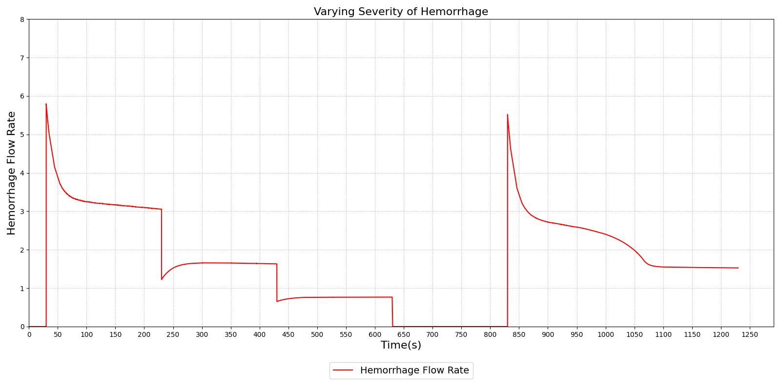
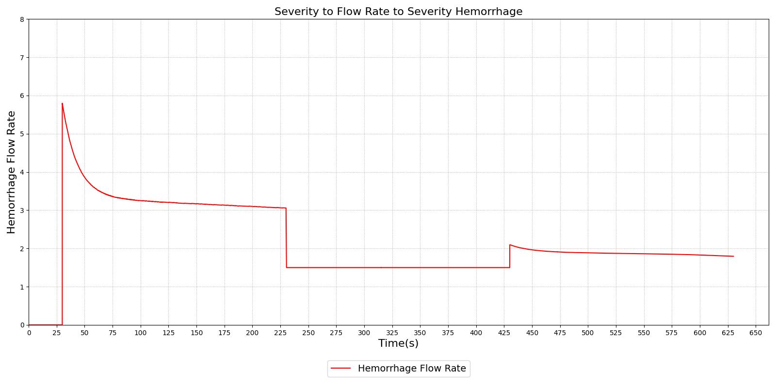
Figure 1 demonstrates the different severity specifications and the impact on the hemorrhage flow rate as the severity is changed or the body responds to the hemorrhage. The results show that the hemorrhage severity changes the flow rate for the hemorrhage as expected, i.e., a 0.5 severity corresponds to 50% of the flow associated with a severity of 1.0. The results also show that as time passes the flow rate will naturally decrease without changing the severity to correspond to the reduction in blood pressure that occurs with hemorrhage. These results also demonstrate the ability to transition from a severity to a flow implementation and back to severity, if required.
|
|
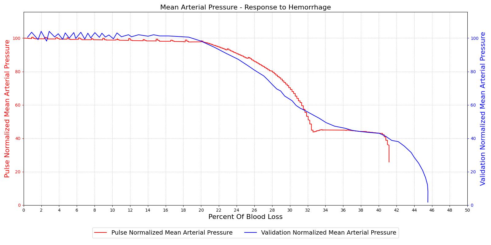
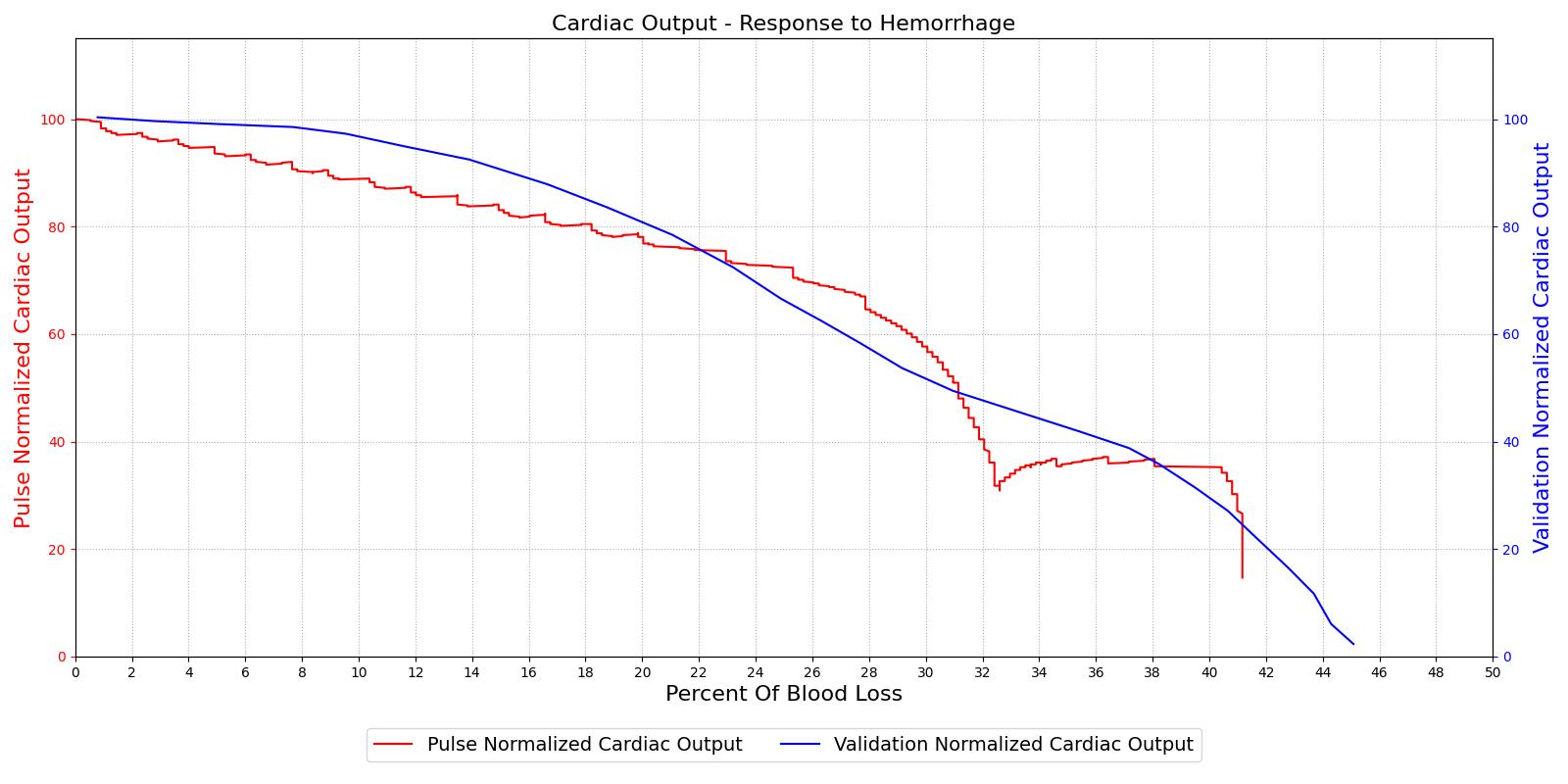
The hemorrhage response was validated with a comparison to the literature. The mean arterial pressure and cardiac output were computed as a function of their baseline value and plotted with the percent blood loss, as shown in Figure 2. The computed results are shown on the left and the validation data [152] is shown on the right.
|
|
For the hemorrhage to shock scenario, our results maintain MAP through a 20% blood loss and CO begins to slowly decrease as expected. At 20%, we see an approximately linear drop in MAP from a as expected compared to experimental data from [152]. The cardiac output shows the correct trend but a larger error for this region. The "last ditch" plateau is then exhibited from a blood loss of just under 35% to just under 45%. The MAP and CO then drop precipitously as expected.
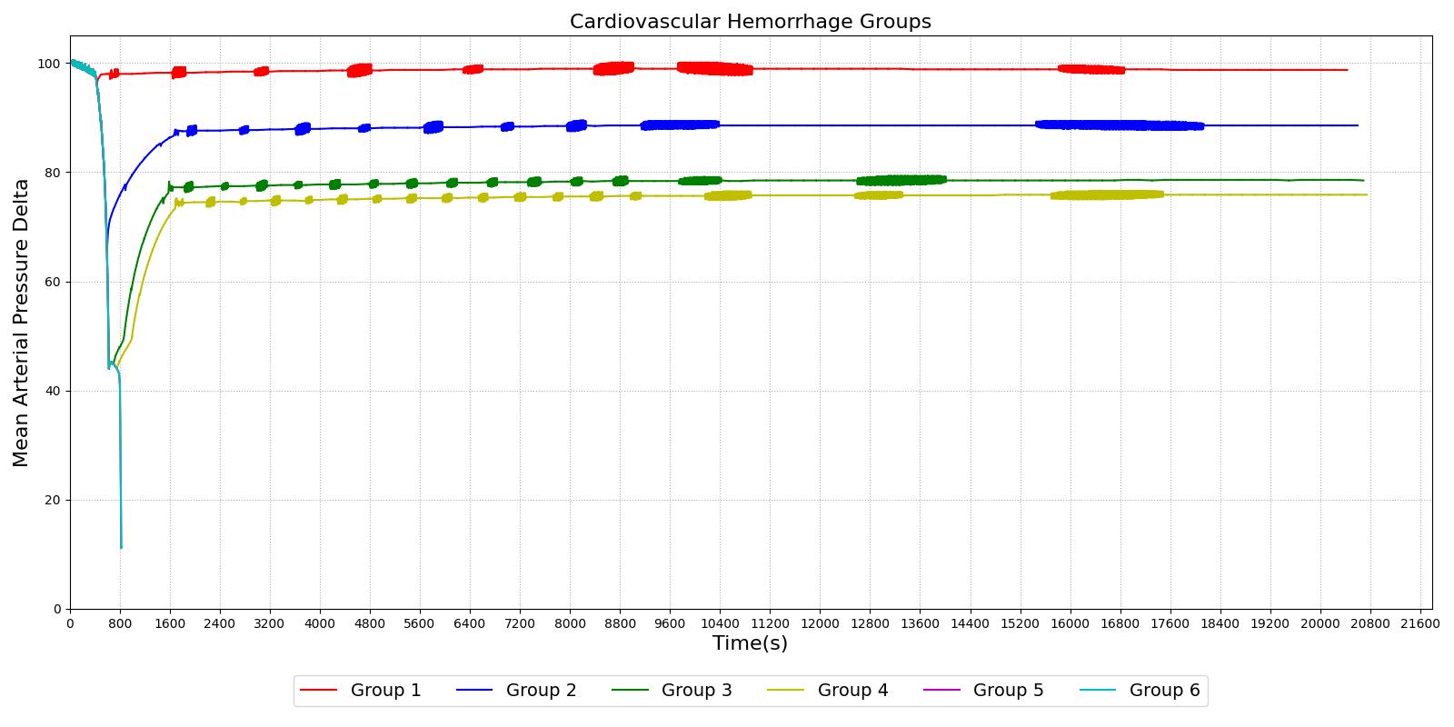
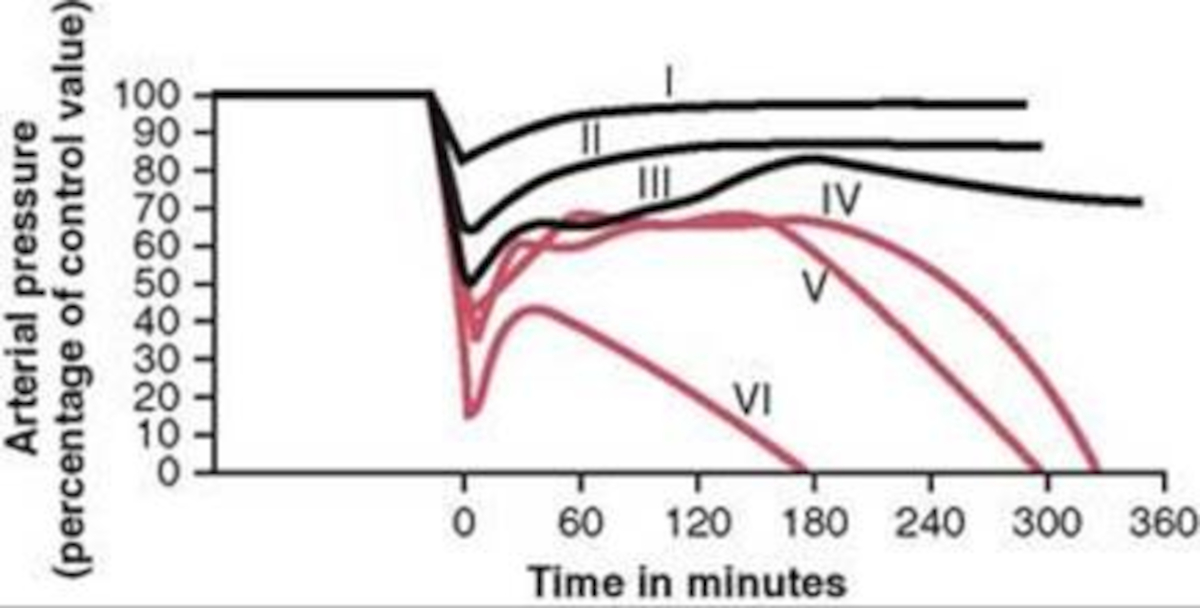
The different types of shock are evident in the data collected for groups of dogs and published in [152]. Groups I, II, and III show cases of nonprogressive shock, Groups IV, and V show cases of progressive shock, and Group VI is an irreversible shock case. The first three groups recover without intervention, the final case leads quickly to death, and the Group IV and V cases show a short rebound before the physiologic decline that occurs without treatment. These cases were duplicated in the Pulse engine. The results and comparison to validation data are shown in Figure 3.
|
|
For the first three group hemorrhage scenarios (90%, 65%, and 50% blood loss), if the hemorrhage is arrested the MAP begins to rise and reaches a stable value. However, for the remaining three scenarios, the hemorrhage is unrecoverable for the patient. This is expected compared to the experimental data and for the degree of shock. However, one limitation of the model is that at the turning point between progressive and irreversible shock, the expected behavior is a temporary recovery lasting minutes to hours followed by deterioration and death. The current model has no ability to reverse the curve once the final deterioration toward deaths occurs. This is triggered at a blood pressure of approximately 40-45 mmHg. While the outcome is the same, the short recovery is not captured. Future work will incorporate this improvement.
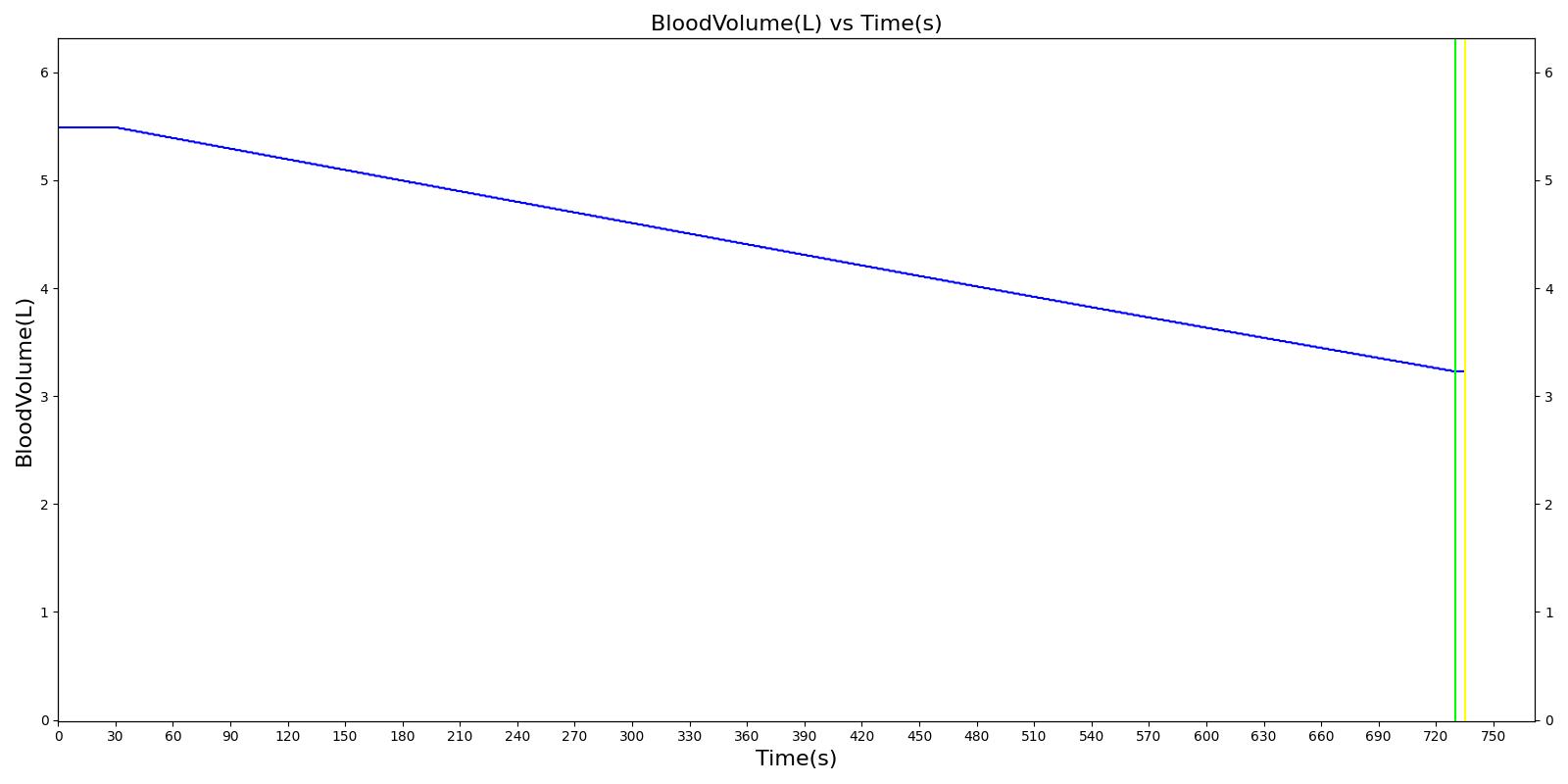
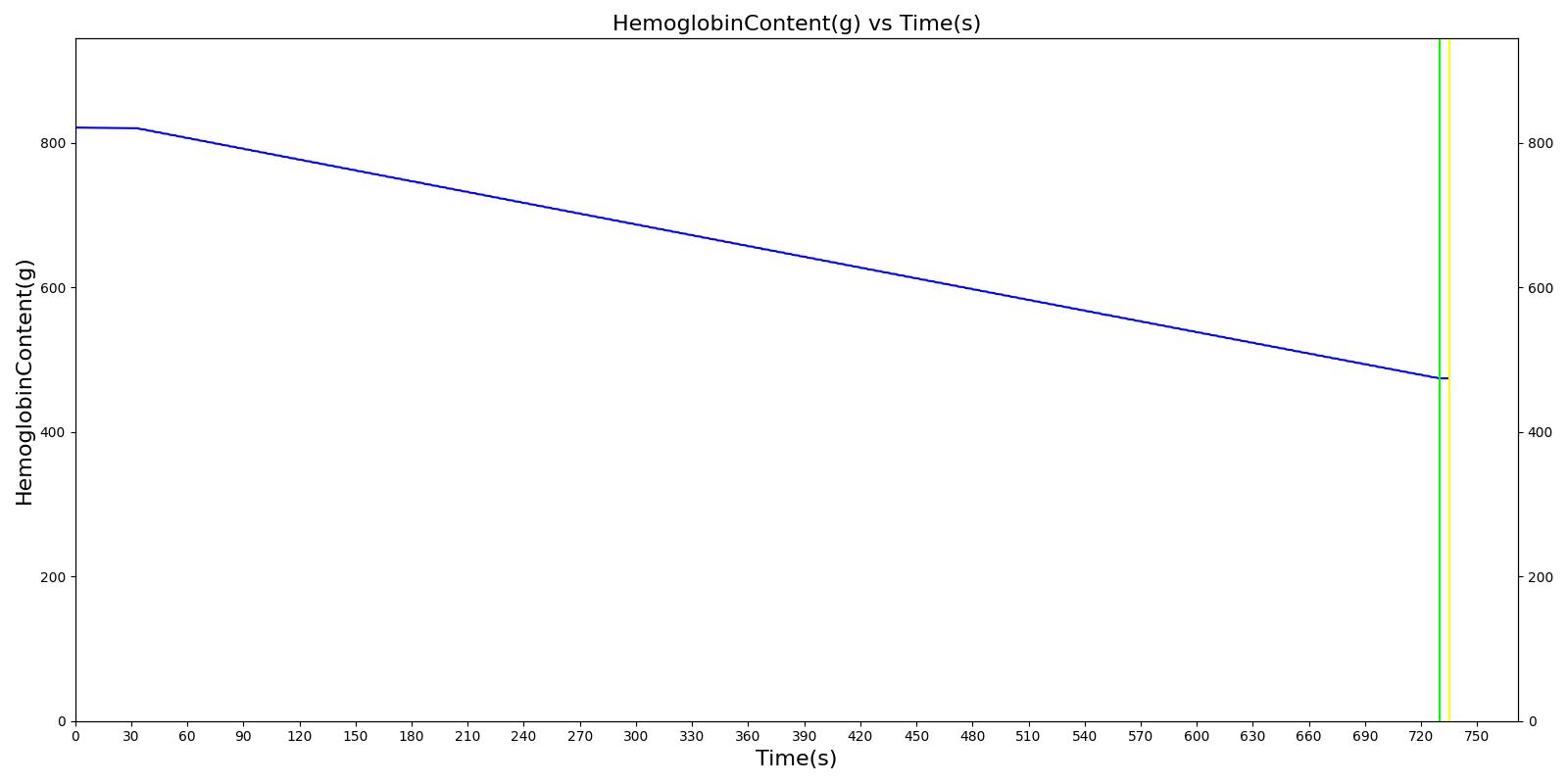
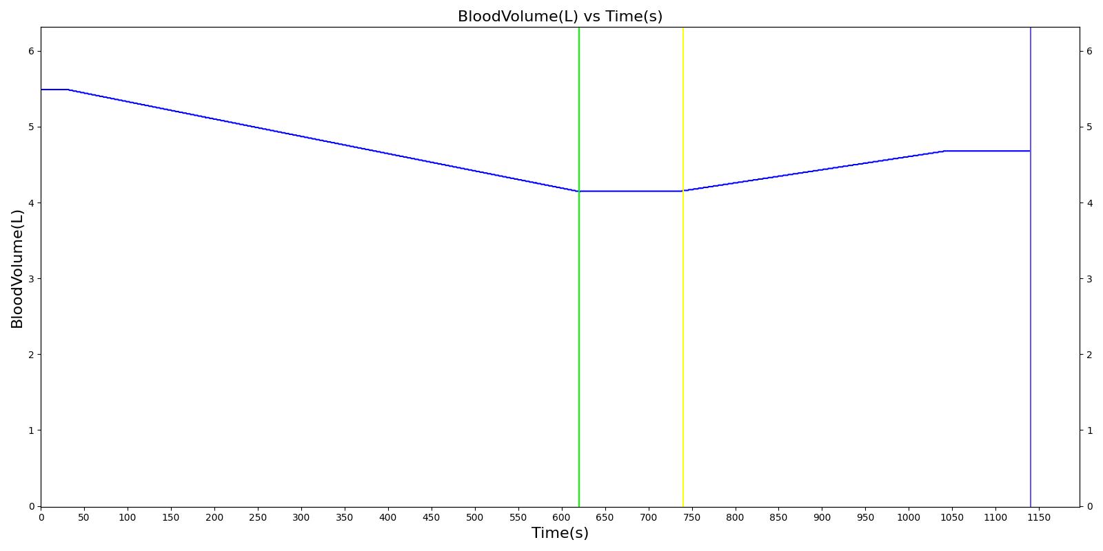
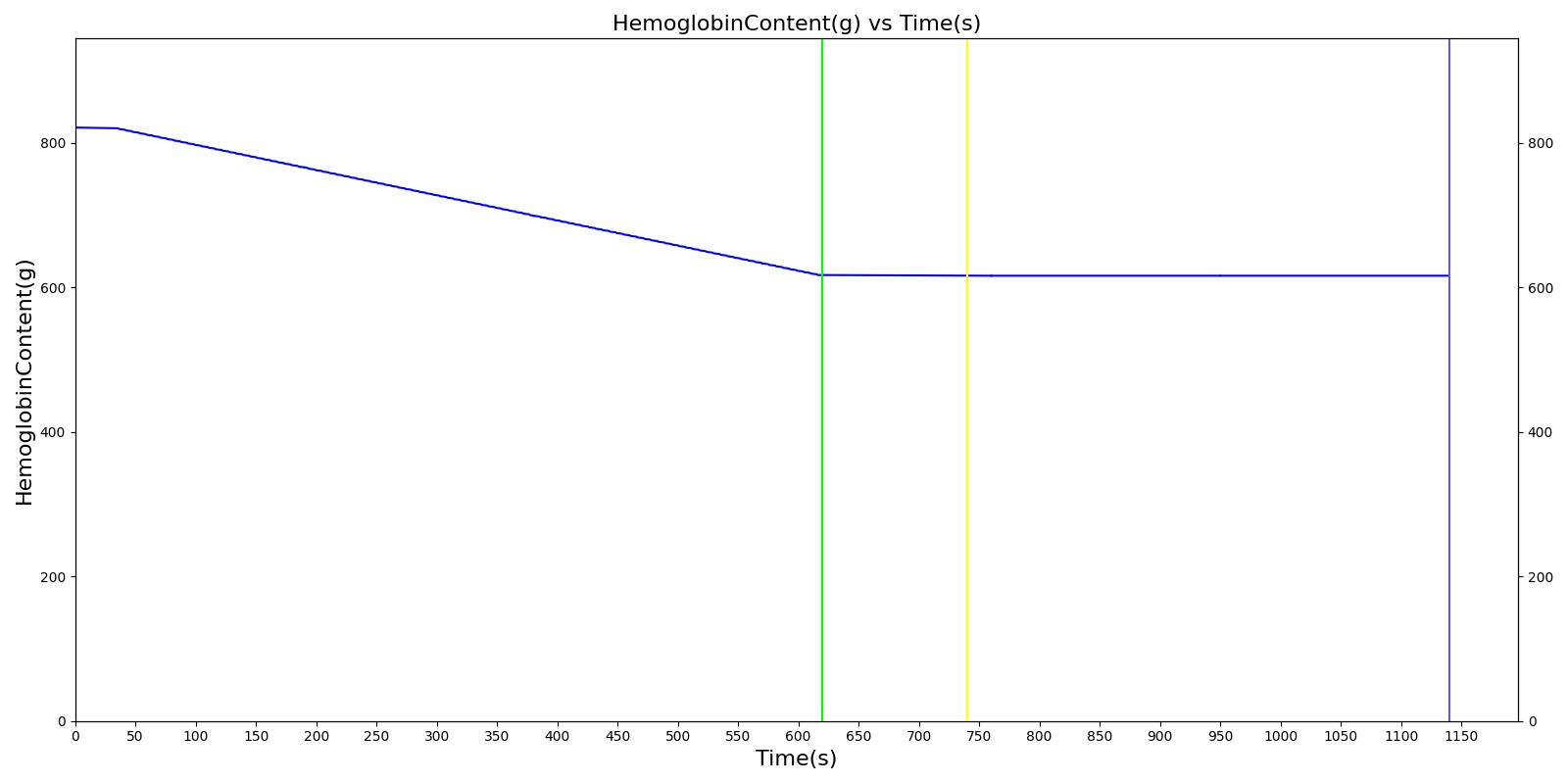
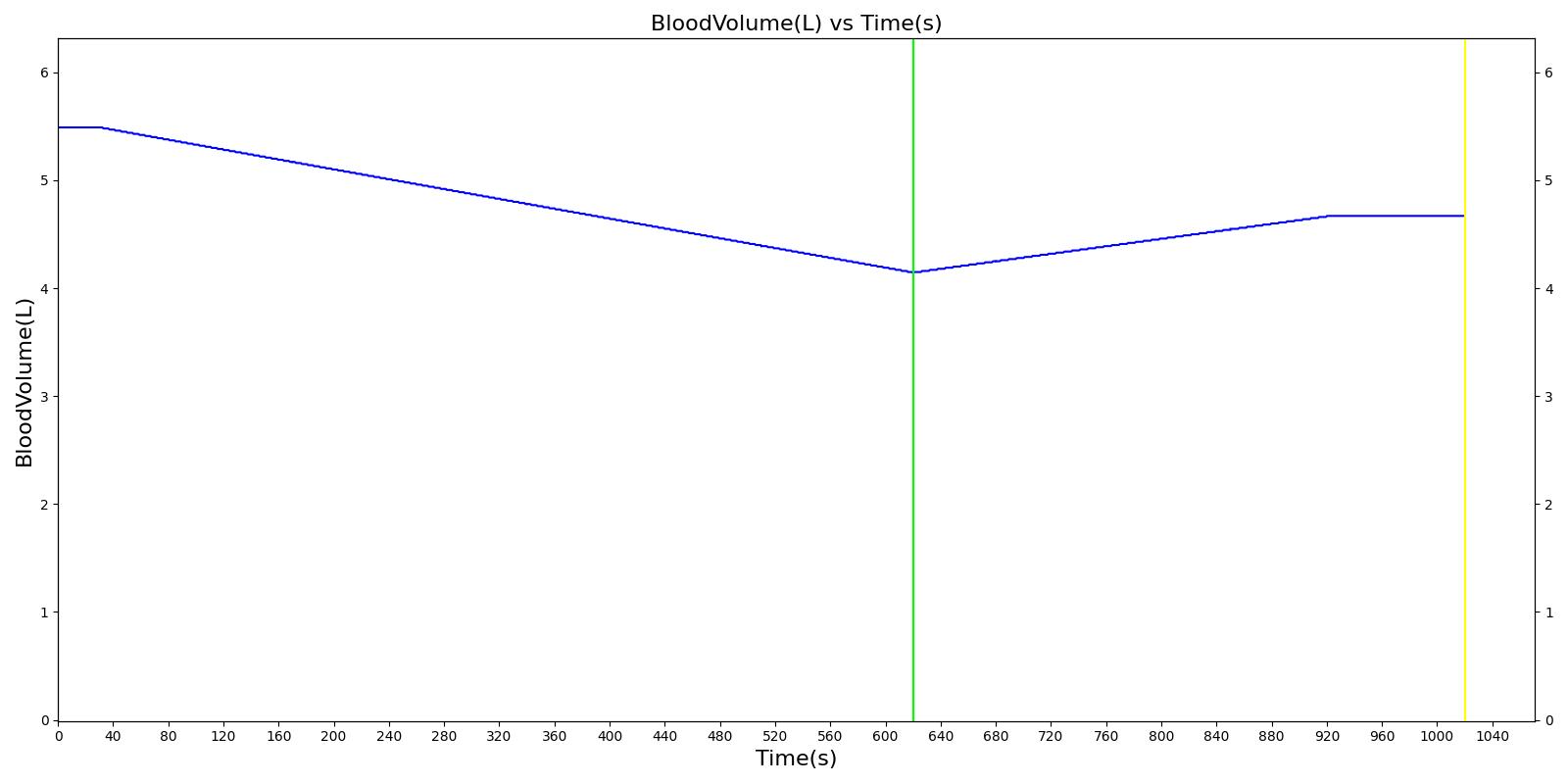
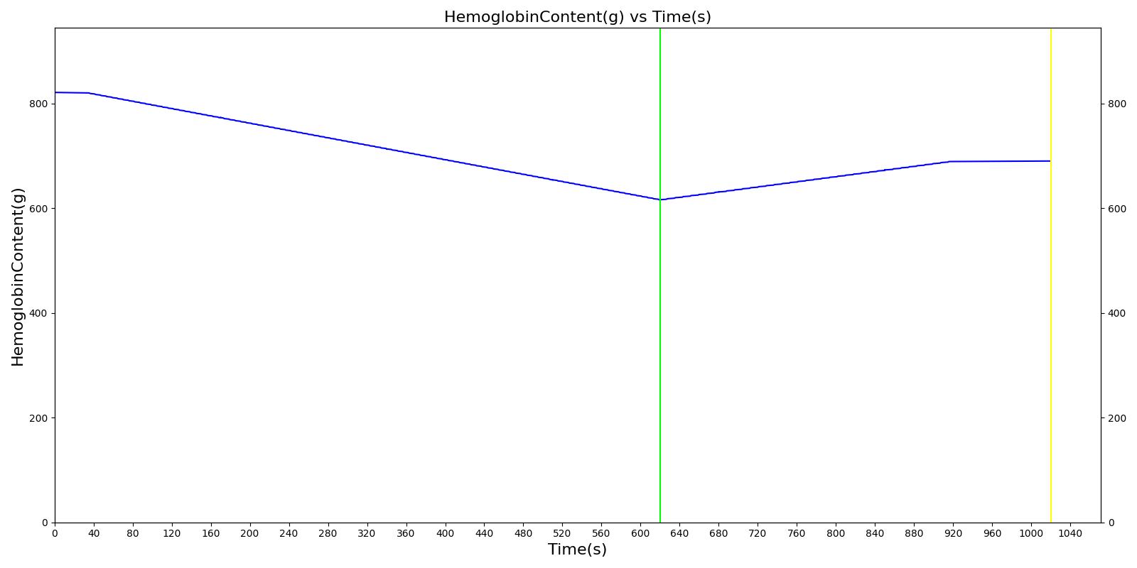
We also saw the expected blood volume, pressure, heart rate, and substance concentration values follow expected trends for the fluid resuscitation scenarios. Figure 4 and Figure 5 show the appropriate substance behavior coupled with the blood volume changes. Like blood volume, the decrease in the substance will be linearly proportional to the bleed rate. For more specific information regarding these substances and their loss due to bleeding, see Blood Chemistry Methodology and Substance Transport Methodology. Figure 4 shows the blood volume and hemoglobin content before, during, and after a massive hemorrhage event with no intervention other than the cessation of hemorrhage. Figure 5 shows a hemorrhage event with subsequent saline administration. Note that the hemoglobin content remains diminished as the blood volume recovers with IV saline. By comparison, Figure 6 shows a scenarios with blood-product intervention and has the hemoglobin increasing with the blood infusion.
|
|
|
|
|
|
|
|
An internal hemorrhage can also be specified for abdominal cardiovascular compartments, including the aorta, vena cava, stomach, splanchnic, spleen, right and left kidneys, large and small intestines, and liver. The internal hemorrhage allows blood to flow into the abdominal cavity, increasing the pressure in the cavity. For the severity implementation, the hemorrhage outlet compartment is specified as the abdominal cavity for Equation 3. This pressure is applied to the aorta, increasing the localized blood pressure as a result of internal blood accumulation. At this time, the internal hemorrhage is only associated with the abdominal region. See the hemothorax model in Respiratory Methodology for details about hemorrhage into the pleural space. In the future, we plan to add functionality for the brain.